2-D Plot for Quantile Regression lines

Description

This function plots quantile regression lines from GLD.lm and one of fun.gld.slope.vary.int.fixed, fun.gld.slope.fixed.int.vary, fun.gld.slope.fixed.int.vary.emp, fun.gld.all.vary.emp, fun.gld.all.vary, fun.gld.slope.vary.int.fixed.emp, GLD.quantreg.

Usage

fun.plot.q(x, y, fit, quant.info, ...)

Arguments

Details

This is intended to plot only two variables, for quantile regression involving more than one explanatory variable, consider plotting the actual values versus fitted values by fitting a secondary GLD quantile model between actual and fitted values.

Value

A graph showing quantile regression lines

Author(s)

Steve Su

References

Su (In Press) "Flexible Parametric Quantile Regression Model" Statistics & Computing

Examples

## Dummy example

## Create dataset

set.seed(10)

x<-rnorm(200,3,2)
y<-3*x+rnorm(200)

dat<-data.frame(y,x)

## Fit FKML GLD regression with 3 simulations

fit<-GLD.lm.full(y~x,data=dat,fun=fun.RMFMKL.ml.m,param="fkml",n.simu=3)

## Find median regression, use empirical method

med.fit<-GLD.quantreg(0.5,fit,slope="fixed",emp=TRUE)

fun.plot.q(x=x,y=y,fit=fit[[1]],med.fit, xlab="x",ylab="y")

## Not run: 

## Plot result of quantile regression

## Extract the Engel dataset 

library(quantreg)
data(engel)

## Fit GLD Regression along with simulations

engel.fit.all<-GLD.lm.full(foodexp~income,data=engel,
param="fmkl",fun=fun.RMFMKL.ml.m)

## Fit quantile regression from 0.1 to 0.9, with equal spacings between 
## quantiles

result<-GLD.quantreg(seq(0.1,.9,length=9),engel.fit.all,intercept="fixed")

## Plot the quantile regression lines

fun.plot.q(x=engel$income,y=engel$foodexp,fit=engel.fit.all[[1]],result,
xlab="income",ylab="Food Expense")

## End(Not run)

Results

R version 3.3.1 (2016-06-21) -- "Bug in Your Hair"
Copyright (C) 2016 The R Foundation for Statistical Computing
Platform: x86_64-pc-linux-gnu (64-bit)

R is free software and comes with ABSOLUTELY NO WARRANTY.
You are welcome to redistribute it under certain conditions.
Type 'license()' or 'licence()' for distribution details.

R is a collaborative project with many contributors.
Type 'contributors()' for more information and
'citation()' on how to cite R or R packages in publications.

Type 'demo()' for some demos, 'help()' for on-line help, or
'help.start()' for an HTML browser interface to help.
Type 'q()' to quit R.

> library(GLDreg)
Loading required package: GLDEX
Loading required package: cluster
> png(filename="/home/ddbj/snapshot/RGM3/R_CC/result/GLDreg/fun.plot.q.Rd_%03d_medium.png", width=480, height=480)
> ### Name: fun.plot.q
> ### Title: 2-D Plot for Quantile Regression lines
> ### Aliases: fun.plot.q
> ### Keywords: hplot
> 
> ### ** Examples
> 
> 
> ## Dummy example
> 
> ## Create dataset
> 
> set.seed(10)
> 
> x<-rnorm(200,3,2)
> y<-3*x+rnorm(200)
> 
> dat<-data.frame(y,x)
> 
> ## Fit FKML GLD regression with 3 simulations
> 
> fit<-GLD.lm.full(y~x,data=dat,fun=fun.RMFMKL.ml.m,param="fkml",n.simu=3)
     [,1]                                                                      
[1,] "This analysis was carried out using FKML GLD"                            
[2,] "The error distribution was estimated using Maximum Likelihood Estimation"
[3,] "The optimisation procedure used was method and it has converged"         
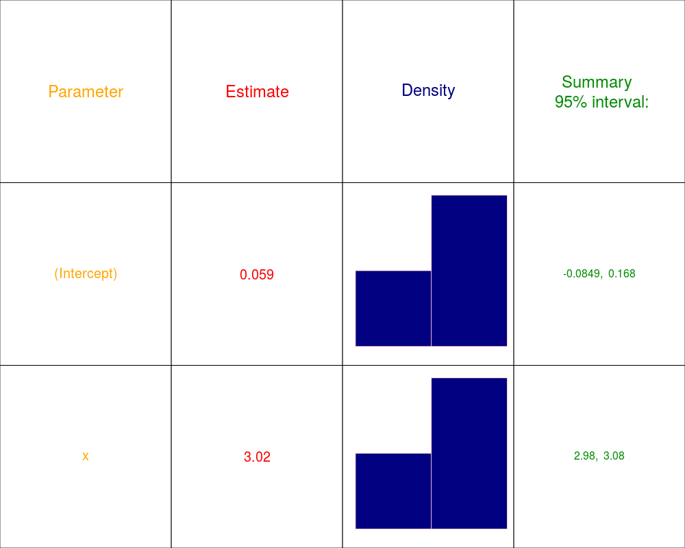
(Intercept)           x          L1          L2          L3          L4 
 0.05895140  3.01981005 -0.01457362  1.29930852  0.22981644  0.20182903 
[1] 1
[1] 2
[1] 3
dev.new(): using pdf(file="Rplots961.pdf")
> 
> ## Find median regression, use empirical method
> 
> med.fit<-GLD.quantreg(0.5,fit,slope="fixed",emp=TRUE)
[1] 0.5
                       0.5
(Intercept)     0.02894985
x               3.01981005
Objective Value 0.00000000
Convergence     0.00000000
> 
> fun.plot.q(x=x,y=y,fit=fit[[1]],med.fit, xlab="x",ylab="y")
[[1]]
NULL

> 
> ## Not run: 
> ##D 
> ##D ## Plot result of quantile regression
> ##D 
> ##D ## Extract the Engel dataset 
> ##D 
> ##D library(quantreg)
> ##D data(engel)
> ##D 
> ##D ## Fit GLD Regression along with simulations
> ##D 
> ##D engel.fit.all<-GLD.lm.full(foodexp~income,data=engel,
> ##D param="fmkl",fun=fun.RMFMKL.ml.m)
> ##D 
> ##D ## Fit quantile regression from 0.1 to 0.9, with equal spacings between 
> ##D ## quantiles
> ##D 
> ##D result<-GLD.quantreg(seq(0.1,.9,length=9),engel.fit.all,intercept="fixed")
> ##D 
> ##D ## Plot the quantile regression lines
> ##D 
> ##D fun.plot.q(x=engel$income,y=engel$foodexp,fit=engel.fit.all[[1]],result,
> ##D xlab="income",ylab="Food Expense")
> ## End(Not run)
> 
> 
> 
> 
> 
> dev.off()
png 
  2 
>