Supported by Dr. Osamu Ogasawara and  . . |
|
Last data update: 2014.03.03 |
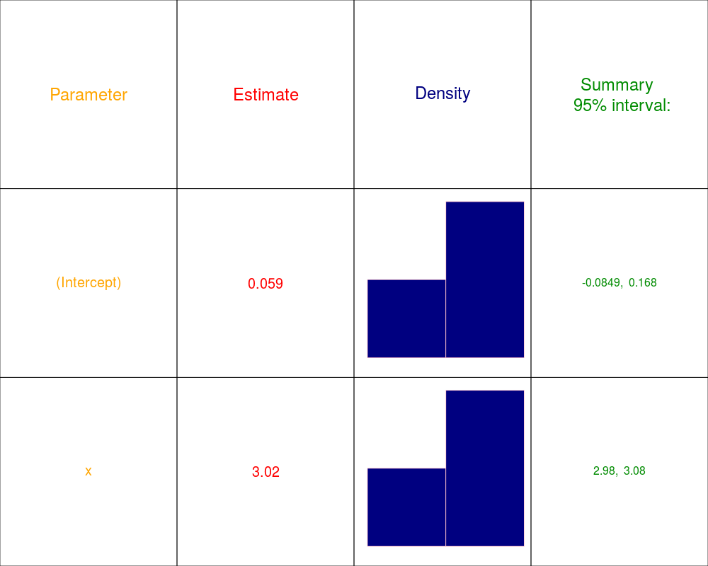
Graphical display of output from
|
overall.fit.obj |
An object from |
alpha |
Specifying the range of interval for the coefficients, default is 0.05, which specifies a 95% interval. |
label |
A character vector indicating the labelling for the coeffiients |
ColourVersion |
Whether to display colour or not, default is TRUE, if set as FALSE, a black and white plot is given. This is only applicable to the coefficient summary graph and has no effect on QQ plots. |
diagnostics |
If TRUE, then QQ plot will be given along with Kolmogorov-Smirnoff test results |
range |
The is the quantile range to plot the QQ plot, defaults to 0.01 and 0.99 to avoid potential problems with extreme values of GLD which might be -Inf or Inf. |
Details
The reason QQ plots are not displayed in black and white even if ColourVersion is set to FALSE is because the colour is necessary in those plots for clarity of display.
Value
Graphics displaying coefficient summary and diagnostic plot (if chosen)
Author(s)
Steve Su
References
Su (In Press) "Flexible Parametric Quantile Regression Model" Statistics & Computing
See Also
GLD.lm.full
Examples
## Dummy example

## Create dataset

set.seed(10)

x<-rnorm(200,3,2)
y<-3*x+rnorm(200)

dat<-data.frame(y,x)

## Fit FKML GLD regression with 3 simulations

fit<-GLD.lm.full(y~x,data=dat,fun=fun.RMFMKL.ml.m,param="fkml",n.simu=3)

## Note this is for illustration only, need to set number
## of simulations around 1000 usually for the graphics below
## to be meaningful

summaryGraphics.gld.lm(fit,ColourVersion=FALSE,diagnostic=FALSE)

## Not run:
## Extract the Engel dataset

library(quantreg)
data(engel)

## Fit a full GLD regression

engel.fit.full<-GLD.lm.full(foodexp~income,data=engel,param="fmkl",
fun=fun.RMFMKL.ml.m)

## Plot coefficient summary

summaryGraphics.gld.lm(engel.fit.full,ColourVersion=FALSE,diagnostic=FALSE)

summaryGraphics.gld.lm(engel.fit.full)

## Extract the mammals dataset
library(MASS)

## Fit a full GLD regression

mammals.fit.full<-GLD.lm.full(log(brain)~log(body),data=mammals,param="fmkl",
fun=fun.RMFMKL.ml.m)

## Plot coefficient summary

summaryGraphics.gld.lm(mammals.fit.full,label=c("intercept","log of body weight"))


## End(Not run)
Results
R version 3.3.1 (2016-06-21) -- "Bug in Your Hair"
Copyright (C) 2016 The R Foundation for Statistical Computing
Platform: x86_64-pc-linux-gnu (64-bit)

R is free software and comes with ABSOLUTELY NO WARRANTY.
You are welcome to redistribute it under certain conditions.
Type 'license()' or 'licence()' for distribution details.

R is a collaborative project with many contributors.
Type 'contributors()' for more information and
'citation()' on how to cite R or R packages in publications.

Type 'demo()' for some demos, 'help()' for on-line help, or
'help.start()' for an HTML browser interface to help.
Type 'q()' to quit R.

> library(GLDreg)
Loading required package: GLDEX
Loading required package: cluster
> png(filename="/home/ddbj/snapshot/RGM3/R_CC/result/GLDreg/summaryGraphics.gld.lm.Rd_%03d_medium.png", width=480, height=480)
> ### Name: summaryGraphics.gld.lm
> ### Title: Graphical display of output from 'GLD.lm.full'
> ### Aliases: summaryGraphics.gld.lm
> ### Keywords: hplot
>
> ### ** Examples
>
>
> ## Dummy example
>
> ## Create dataset
>
> set.seed(10)
>
> x<-rnorm(200,3,2)
> y<-3*x+rnorm(200)
>
> dat<-data.frame(y,x)
>
> ## Fit FKML GLD regression with 3 simulations
>
> fit<-GLD.lm.full(y~x,data=dat,fun=fun.RMFMKL.ml.m,param="fkml",n.simu=3)
     [,1]
[1,] "This analysis was carried out using FKML GLD"
[2,] "The error distribution was estimated using Maximum Likelihood Estimation"
[3,] "The optimisation procedure used was method and it has converged"
(Intercept)           x          L1          L2          L3          L4
 0.05895140  3.01981005 -0.01457362  1.29930852  0.22981644  0.20182903
[1] 1
[1] 2
[1] 3
dev.new(): using pdf(file="Rplots963.pdf")
>
> ## Note this is for illustration only, need to set number
> ## of simulations around 1000 usually for the graphics below
> ## to be meaningful
>
> summaryGraphics.gld.lm(fit,ColourVersion=FALSE,diagnostic=FALSE)
>
> ## Not run:
> ##D ## Extract the Engel dataset
> ##D
> ##D library(quantreg)
> ##D data(engel)
> ##D
> ##D ## Fit a full GLD regression
> ##D
> ##D engel.fit.full<-GLD.lm.full(foodexp~income,data=engel,param="fmkl",
> ##D fun=fun.RMFMKL.ml.m)
> ##D
> ##D ## Plot coefficient summary
> ##D
> ##D summaryGraphics.gld.lm(engel.fit.full,ColourVersion=FALSE,diagnostic=FALSE)
> ##D
> ##D summaryGraphics.gld.lm(engel.fit.full)
> ##D
> ##D ## Extract the mammals dataset
> ##D library(MASS)
> ##D
> ##D ## Fit a full GLD regression
> ##D
> ##D mammals.fit.full<-GLD.lm.full(log(brain)~log(body),data=mammals,param="fmkl",
> ##D fun=fun.RMFMKL.ml.m)
> ##D
> ##D ## Plot coefficient summary
> ##D
> ##D summaryGraphics.gld.lm(mammals.fit.full,label=c("intercept","log of body weight"))
> ##D
> ## End(Not run)
>
>
>
>
>
> dev.off()
png
  2
>
|