R Graphical Manual

Browse All

Last data update: 2014.03.03

R: Unsupervised clustering using a general GMCM

fit.full.GMCM

R Documentation

Unsupervised clustering using a general GMCM

Description

Perform unsupervised clustering using various optimization procedures to find the maximum likelihood estimate of the general Gaussian mixture copula model by Tewari et al. (2011).

Usage

fit.full.GMCM(u, m, theta = choose.theta(u, m), method = c("NM", "SANN",
  "L-BFGS", "L-BFGS-B", "PEM"), max.ite = 1000, verbose = TRUE, ...)

Arguments

`u`	An `n` by `d` matrix of ranked and scaled test statistics. Rows correspond to observations and columns to the dimensions of the variables.
`m`	The number of components to be fitted.
`theta`	A list of parameters as defined in `rtheta`. If `theta` is not provided, then heuristic starting values are chosen using the k-means algorithm.
`method`	A character vector of length 1. The optimization method used. Should be either `"NM"`, `"SANN"`, `"L-BFGS"`, `"L-BFGS-B"`, or `"PEM"` which are the Nelder-Mead, Simulated Annealing, limited-memory quasi-Newton method, limited-memory quasi-Newton method with box constraints, and the pseudo EM algorithm, respectively. Default is `"NM"`. See `optim` for further details.
`max.ite`	The maximum number of iterations. If the `method` is `"SANN"` this is the number of iterations as there is no other stopping criterion. (See `optim`)
`verbose`	Logical. If `TRUE`, a trace of the parameter estimates is made.
`...`	Arguments passed to the `control`-list in `optim` or `PseudoEMAlgorithm` if the `method` is `"PEM"`.

Details

The "L-BFGS-B" method does not perform a transformation of the parameters and uses box constraints as implemented in optim.
Note that the many parameter configurations are poorly estimable or directly unidentifiable.

Value

A list of parameters formatted as described in rtheta.

Note

All the optimization procedures are strongly dependent on the initial values and the cooling scheme. Therefore it is advisable to apply multiple different initial parameters and select the best fit.

The choose.theta itself chooses random a initialization. Hence, the output when theta is not directly supplied can vary.

See optim for further details.

Author(s)

Anders Ellern Bilgrau <anders.ellern.bilgrau@gmail.com>

References

Li, Q., Brown, J. B. J. B., Huang, H., & Bickel, P. J. (2011). Measuring reproducibility of high-throughput experiments. The Annals of Applied Statistics, 5(3), 1752-1779. doi:10.1214/11-AOAS466

Tewari, A., Giering, M. J., & Raghunathan, A. (2011). Parametric Characterization of Multimodal Distributions with Non-gaussian Modes. 2011 IEEE 11th International Conference on Data Mining Workshops, 286-292. doi:10.1109/ICDMW.2011.135

Examples

set.seed(17)
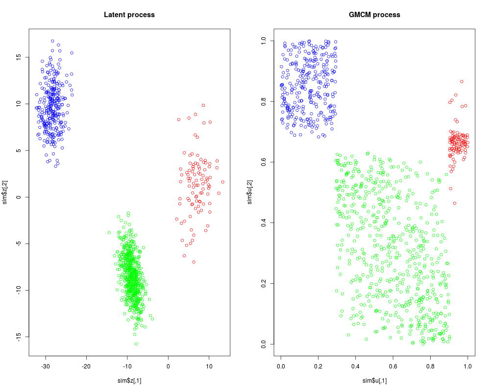
sim <- SimulateGMCMData(n = 1000, m = 3, d = 2)

# Plotting simulated data
par(mfrow = c(1,2))
plot(sim$z, col = rainbow(3)[sim$K], main = "Latent process")
plot(sim$u, col = rainbow(3)[sim$K], main = "GMCM process")

# Observed data
uhat <- Uhat(sim$u)

# The model should be fitted multiple times using different starting estimates
start.theta <- choose.theta(uhat, m = 3)  # Random starting estimate
res <- fit.full.GMCM(u = uhat, theta = start.theta,
                     method = "NM", max.ite = 3000,
                     reltol = 1e-2, trace = TRUE)  # Note, 1e-2 is too big

# Confusion matrix
Khat <- apply(get.prob(uhat, theta = res), 1, which.max)
table("Khat" = Khat, "K" = sim$K)  # Note, some components have been swapped

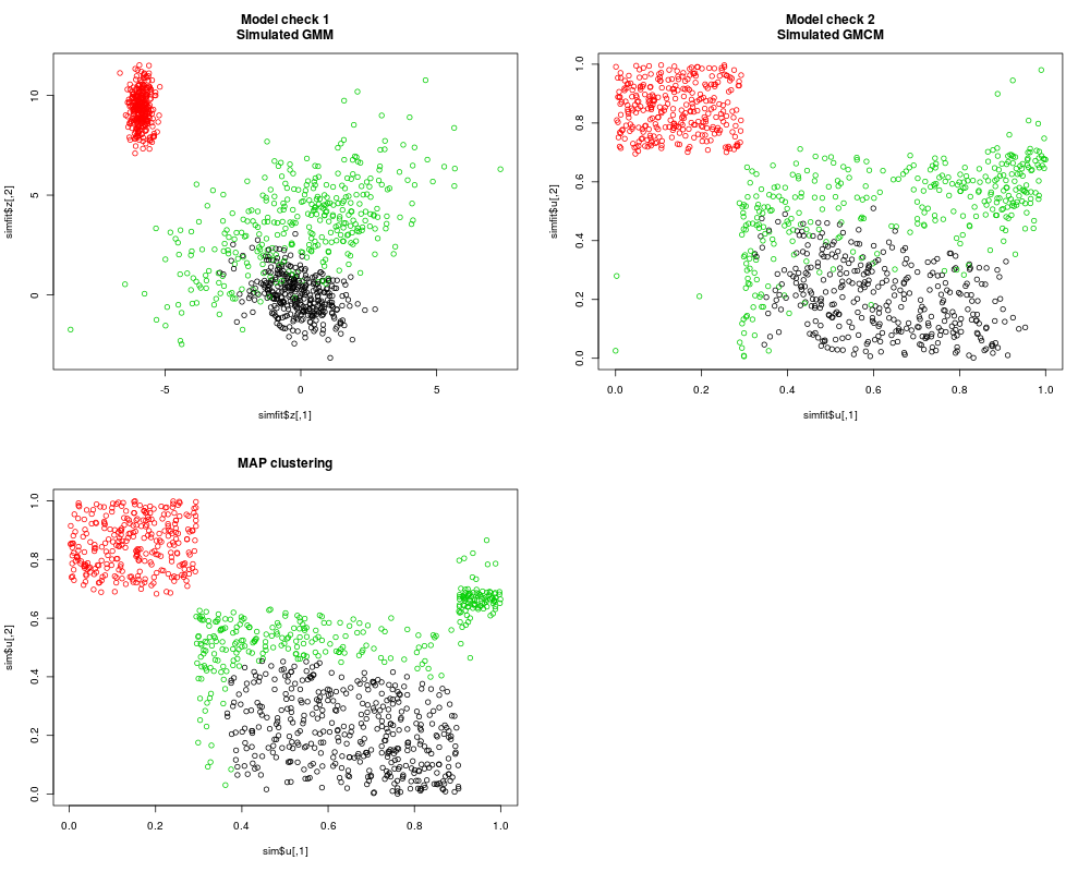
# Simulation from GMCM with the fitted parameters
simfit <- SimulateGMCMData(n = 1000, theta = res)

# As seen, the underlying latent process is hard to estimate.
# The clustering, however, is very good.
par(mfrow = c(2,2))
plot(simfit$z, col = simfit$K, main = "Model check 1\nSimulated GMM")
plot(simfit$u, col = simfit$K, main = "Model check 2\nSimulated GMCM")
plot(sim$u, col = Khat, main = "MAP clustering")

Results


R version 3.3.1 (2016-06-21) -- "Bug in Your Hair"
Copyright (C) 2016 The R Foundation for Statistical Computing
Platform: x86_64-pc-linux-gnu (64-bit)

R is free software and comes with ABSOLUTELY NO WARRANTY.
You are welcome to redistribute it under certain conditions.
Type 'license()' or 'licence()' for distribution details.

R is a collaborative project with many contributors.
Type 'contributors()' for more information and
'citation()' on how to cite R or R packages in publications.

Type 'demo()' for some demos, 'help()' for on-line help, or
'help.start()' for an HTML browser interface to help.
Type 'q()' to quit R.

> library(GMCM)
> png(filename="/home/ddbj/snapshot/RGM3/R_CC/result/GMCM/fit.full.GMCM.Rd_%03d_medium.png", width=480, height=480)
> ### Name: fit.full.GMCM
> ### Title: Unsupervised clustering using a general GMCM
> ### Aliases: fit.full.GMCM fit.full.gmcm
> 
> ### ** Examples
> 
> set.seed(17)
> sim <- SimulateGMCMData(n = 1000, m = 3, d = 2)
> 
> # Plotting simulated data
> par(mfrow = c(1,2))
> plot(sim$z, col = rainbow(3)[sim$K], main = "Latent process")
> plot(sim$u, col = rainbow(3)[sim$K], main = "GMCM process")
> 
> # Observed data
> uhat <- Uhat(sim$u)
> 
> # The model should be fitted multiple times using different starting estimates
> start.theta <- choose.theta(uhat, m = 3)  # Random starting estimate
> res <- fit.full.GMCM(u = uhat, theta = start.theta,
+                      method = "NM", max.ite = 3000,
+                      reltol = 1e-2, trace = TRUE)  # Note, 1e-2 is too big
  Nelder-Mead direct search function minimizer
function value for initial parameters = -532.119142
  Scaled convergence tolerance is 5.32129
Stepsize computed as 0.908776
BUILD             15 592.493941 -579.264880
LO-REDUCTION      17 -191.688195 -579.264880
HI-REDUCTION      19 -199.665759 -579.264880
LO-REDUCTION      21 -248.049142 -579.264880
HI-REDUCTION      23 -366.700910 -579.264880
LO-REDUCTION      25 -409.223490 -599.883027
HI-REDUCTION      27 -444.829521 -599.883027
LO-REDUCTION      29 -468.981142 -599.883027
HI-REDUCTION      31 -478.942797 -599.883027
HI-REDUCTION      33 -490.506246 -599.883027
HI-REDUCTION      35 -491.956415 -599.883027
LO-REDUCTION      37 -492.921066 -599.883027
LO-REDUCTION      39 -498.905480 -599.883027
LO-REDUCTION      41 -501.658194 -599.883027
LO-REDUCTION      43 -532.119142 -599.883027
REFLECTION        45 -532.136454 -608.618017
REFLECTION        47 -534.236088 -615.759559
REFLECTION        49 -536.789234 -619.299238
REFLECTION        51 -546.483086 -621.685781
LO-REDUCTION      53 -553.068460 -621.685781
LO-REDUCTION      55 -562.123324 -621.920152
REFLECTION        57 -567.269898 -621.942192
REFLECTION        59 -569.794759 -646.618172
LO-REDUCTION      61 -572.583502 -646.618172
REFLECTION        63 -579.264880 -650.581081
HI-REDUCTION      65 -579.525220 -650.581081
LO-REDUCTION      67 -594.625222 -650.581081
LO-REDUCTION      69 -597.572392 -650.581081
REFLECTION        71 -599.883027 -659.641852
LO-REDUCTION      73 -608.618017 -659.641852
EXTENSION         75 -612.150562 -676.993643
LO-REDUCTION      77 -615.759559 -676.993643
LO-REDUCTION      79 -619.299238 -676.993643
LO-REDUCTION      81 -619.394835 -676.993643
LO-REDUCTION      83 -621.685781 -676.993643
LO-REDUCTION      85 -621.920152 -676.993643
LO-REDUCTION      87 -621.942192 -676.993643
LO-REDUCTION      89 -631.953485 -676.993643
LO-REDUCTION      91 -637.615680 -676.993643
REFLECTION        93 -646.230967 -680.065226
LO-REDUCTION      95 -646.618172 -680.065226
HI-REDUCTION      97 -647.294905 -680.065226
LO-REDUCTION      99 -647.588391 -680.065226
LO-REDUCTION     101 -650.581081 -680.065226
LO-REDUCTION     103 -656.503424 -680.065226
REFLECTION       105 -656.781239 -680.659019
EXTENSION        107 -659.171445 -692.865079
LO-REDUCTION     109 -659.641852 -692.865079
LO-REDUCTION     111 -660.059119 -692.865079
LO-REDUCTION     113 -662.495231 -692.865079
REFLECTION       115 -671.164238 -693.389412
LO-REDUCTION     117 -671.586443 -693.389412
LO-REDUCTION     119 -672.763716 -693.389412
REFLECTION       121 -673.959931 -694.622827
LO-REDUCTION     123 -674.219436 -694.622827
REFLECTION       125 -675.482792 -700.502234
LO-REDUCTION     127 -675.999163 -700.502234
LO-REDUCTION     129 -676.993643 -700.502234
LO-REDUCTION     131 -680.065226 -700.502234
EXTENSION        133 -680.659019 -705.882619
LO-REDUCTION     135 -684.971455 -705.882619
EXTENSION        137 -685.973558 -707.846676
LO-REDUCTION     139 -688.335078 -707.846676
EXTENSION        141 -689.992120 -711.883730
LO-REDUCTION     143 -690.725193 -711.883730
LO-REDUCTION     145 -692.814691 -711.883730
LO-REDUCTION     147 -692.865079 -711.883730
HI-REDUCTION     149 -693.015372 -711.883730
LO-REDUCTION     151 -693.389412 -711.883730
LO-REDUCTION     153 -693.953910 -711.883730
REFLECTION       155 -694.622827 -715.529357
LO-REDUCTION     157 -697.680840 -715.529357
HI-REDUCTION     159 -700.502234 -715.529357
LO-REDUCTION     161 -701.370441 -715.529357
LO-REDUCTION     163 -701.380084 -715.529357
HI-REDUCTION     165 -702.801125 -715.529357
LO-REDUCTION     167 -705.695891 -715.529357
LO-REDUCTION     169 -705.882619 -716.427646
LO-REDUCTION     171 -707.297957 -716.427646
REFLECTION       173 -707.846676 -718.113527
HI-REDUCTION     175 -708.346704 -718.113527
LO-REDUCTION     177 -708.849320 -718.113527
HI-REDUCTION     179 -711.639995 -718.113527
LO-REDUCTION     181 -711.787184 -718.113527
LO-REDUCTION     183 -711.859122 -718.113527
REFLECTION       185 -711.883730 -718.215761
LO-REDUCTION     187 -712.044354 -718.215761
LO-REDUCTION     189 -712.446052 -718.215761
LO-REDUCTION     191 -712.973631 -718.463450
Exiting from Nelder Mead minimizer
    193 function evaluations used
> 
> # Confusion matrix
> Khat <- apply(get.prob(uhat, theta = res), 1, which.max)
> table("Khat" = Khat, "K" = sim$K)  # Note, some components have been swapped
    K
Khat   1   2   3
   1   0 403   0
   2   0   0 293
   3  97 207   0
> 
> # Simulation from GMCM with the fitted parameters
> simfit <- SimulateGMCMData(n = 1000, theta = res)
> 
> # As seen, the underlying latent process is hard to estimate.
> # The clustering, however, is very good.
> par(mfrow = c(2,2))
> plot(simfit$z, col = simfit$K, main = "Model check 1\nSimulated GMM")
> plot(simfit$u, col = simfit$K, main = "Model check 2\nSimulated GMCM")
> plot(sim$u, col = Khat, main = "MAP clustering")
> 
> 
> 
> 
> 
> dev.off()
null device 
          1 
>