R Graphical Manual

Browse All

Last data update: 2014.03.03

R: Reproducibility/meta analysis using GMCMs

fit.meta.GMCM

R Documentation

Reproducibility/meta analysis using GMCMs

Description

This function performs reproducibility (or meta) analysis using GMCMs. It features various optimization routines to identify the maximum likelihood estimate of the special Gaussian mixture copula model proposed by Li et. al. (2011).

Usage

fit.meta.GMCM(u, init.par, method = c("NM", "SANN", "L-BFGS", "L-BFGS-B",
  "PEM"), max.ite = 1000, verbose = TRUE, positive.rho = TRUE,
  trace.theta = FALSE, ...)

Arguments

`u`	An `n` by `d` matrix of test statistics. Rows correspond to features and columns to experiments. Large values are assumed to be indicative of reproducible genes.
`init.par`	A 4-dimensional vector of the initial parameters where, `init.par[1]` is the mixture proportion of spurious signals, `init.par[2]` is the mean, `init.par[3]` is the standard deviation, `init.par[4]` is the correlation.
`method`	A character vector of length 1. The optimization method used. Should be either `"NM"`, `"SANN"`, `"L-BFGS"`, `"L-BFGS-B"`, or `"PEM"` which are abbreviations of Nelder-Mead, Simulated Annealing, limited-memory quasi-Newton method, limited-memory quasi-Newton method with box constraints, and the pseudo EM algorithm, respectively. Default is `"NM"`. See `optim` for further details.
`max.ite`	The maximum number of iterations. If the `method` is `"SANN"` this is the number of iterations as there is no other stopping criterion. (See `optim`)
`verbose`	Logical. If `TRUE`, the log-likelihood values are printed.
`positive.rho`	`logical`. If `TRUE`, the correlation parameter is restricted to be positive.
`trace.theta`	`logical`. Extra convergence information is appended as a list to the output returned if `TRUE`. The exact behavior is dependent on the value of `method`. If `method` equals `"PEM"`, the argument is passed to `trace.theta` in `PseudoEMAlgorithm`. Otherwise it is passed to the control argument `trace` in `optim`.
`...`	Arguments passed to the `control`-list in `optim` or `PseudoEMAlgorithm` if `method` is `"PEM"`.

Details

The "L-BFGS-B" method does not perform a transformation of the parameters.

Value

A vector par of length 4 of the fitted parameters where par[1] is the probability of being from the first (or null) component, par[2] is the mean, par[3] is the standard deviation, and par[4] is the correlation.

Note

Simulated annealing is strongly dependent on the initial values and the cooling scheme.

See optim for further details.

Author(s)

Anders Ellern Bilgrau <anders.ellern.bilgrau@gmail.com>

References

Li, Q., Brown, J. B. J. B., Huang, H., & Bickel, P. J. (2011). Measuring reproducibility of high-throughput experiments. The Annals of Applied Statistics, 5(3), 1752-1779. doi:10.1214/11-AOAS466

Examples

set.seed(1)

# True parameters
true.par <- c(0.9, 2, 0.7, 0.6)
# Simulation of data from the GMCM model
data <- SimulateGMCMData(n = 1000, par = true.par)
uhat <- Uhat(data$u) # Ranked observed data

init.par <- c(0.5, 1, 0.5, 0.9)  # Initial parameters

# Optimization with Nelder-Mead
nm.par   <- fit.meta.GMCM(uhat, init.par = init.par, method = "NM")

## Not run: 
# Comparison with other optimization methods
# Optimization with simulated annealing
sann.par <- fit.meta.GMCM(uhat, init.par = init.par, method = "SANN",
                          max.ite = 3000, temp = 1)
# Optimization with the Pseudo EM algorithm
pem.par  <- fit.meta.GMCM(uhat, init.par = init.par, method = "PEM")

# The estimates agree nicely
rbind("True" = true.par, "Start" = init.par,
      "NM" = nm.par, "SANN" = sann.par, "PEM" = pem.par)

## End(Not run)

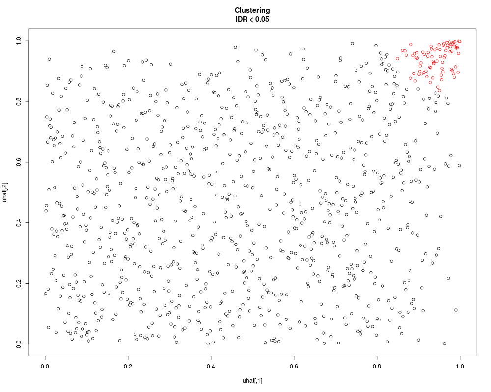
# Get estimated cluster
Khat <- get.IDR(x = uhat, par = nm.par)$Khat
plot(uhat, col = Khat, main = "Clustering\nIDR < 0.05")

Results


R version 3.3.1 (2016-06-21) -- "Bug in Your Hair"
Copyright (C) 2016 The R Foundation for Statistical Computing
Platform: x86_64-pc-linux-gnu (64-bit)

R is free software and comes with ABSOLUTELY NO WARRANTY.
You are welcome to redistribute it under certain conditions.
Type 'license()' or 'licence()' for distribution details.

R is a collaborative project with many contributors.
Type 'contributors()' for more information and
'citation()' on how to cite R or R packages in publications.

Type 'demo()' for some demos, 'help()' for on-line help, or
'help.start()' for an HTML browser interface to help.
Type 'q()' to quit R.

> library(GMCM)
> png(filename="/home/ddbj/snapshot/RGM3/R_CC/result/GMCM/fit.meta.GMCM.Rd_%03d_medium.png", width=480, height=480)
> ### Name: fit.meta.GMCM
> ### Title: Reproducibility/meta analysis using GMCMs
> ### Aliases: fit.meta.GMCM fit.meta.gmcm
> 
> ### ** Examples
> 
> set.seed(1)
> 
> # True parameters
> true.par <- c(0.9, 2, 0.7, 0.6)
> # Simulation of data from the GMCM model
> data <- SimulateGMCMData(n = 1000, par = true.par)
> uhat <- Uhat(data$u) # Ranked observed data
> 
> init.par <- c(0.5, 1, 0.5, 0.9)  # Initial parameters
> 
> # Optimization with Nelder-Mead
> nm.par   <- fit.meta.GMCM(uhat, init.par = init.par, method = "NM")
  Nelder-Mead direct search function minimizer
function value for initial parameters = 176.343401
  Scaled convergence tolerance is 2.62772e-06
Stepsize computed as 0.219722
BUILD              5 226.656977 105.973352
LO-REDUCTION       7 215.745222 105.973352
EXTENSION          9 176.343401 4.976728
LO-REDUCTION      11 133.560182 4.976728
EXTENSION         13 114.710466 -45.512205
EXTENSION         15 105.973352 -86.690136
EXTENSION         17 11.976424 -97.922305
LO-REDUCTION      19 4.976728 -97.922305
LO-REDUCTION      21 -45.512205 -97.922305
LO-REDUCTION      23 -78.907712 -97.922305
REFLECTION        25 -86.690136 -105.072127
LO-REDUCTION      27 -95.841590 -105.072127
LO-REDUCTION      29 -97.114144 -105.072127
LO-REDUCTION      31 -97.922305 -105.072127
LO-REDUCTION      33 -99.021762 -105.072127
LO-REDUCTION      35 -102.447782 -105.072127
EXTENSION         37 -102.566757 -109.005176
HI-REDUCTION      39 -103.544631 -109.005176
LO-REDUCTION      41 -105.010085 -109.005176
EXTENSION         43 -105.072127 -111.555517
LO-REDUCTION      45 -105.494019 -111.555517
EXTENSION         47 -107.926302 -114.706877
LO-REDUCTION      49 -108.163783 -114.706877
LO-REDUCTION      51 -109.005176 -114.706877
REFLECTION        53 -111.555517 -115.585400
HI-REDUCTION      55 -113.529332 -115.585400
LO-REDUCTION      57 -113.796380 -115.585400
EXTENSION         59 -113.979420 -116.852099
HI-REDUCTION      61 -114.706877 -116.852099
LO-REDUCTION      63 -115.194526 -116.852099
EXTENSION         65 -115.255631 -117.583240
HI-REDUCTION      67 -115.585400 -117.583240
EXTENSION         69 -116.276863 -118.192081
LO-REDUCTION      71 -116.284681 -118.192081
REFLECTION        73 -116.852099 -118.328874
LO-REDUCTION      75 -117.583240 -118.387443
LO-REDUCTION      77 -117.737665 -118.387443
HI-REDUCTION      79 -118.192081 -118.387443
HI-REDUCTION      81 -118.204023 -118.387443
HI-REDUCTION      83 -118.294593 -118.387443
LO-REDUCTION      85 -118.325318 -118.387443
REFLECTION        87 -118.328874 -118.401466
LO-REDUCTION      89 -118.331957 -118.401466
LO-REDUCTION      91 -118.368285 -118.401466
REFLECTION        93 -118.387443 -118.405678
EXTENSION         95 -118.396046 -118.435327
HI-REDUCTION      97 -118.398167 -118.435327
HI-REDUCTION      99 -118.401466 -118.435327
EXTENSION        101 -118.405678 -118.467822
LO-REDUCTION     103 -118.417378 -118.467822
LO-REDUCTION     105 -118.418910 -118.467822
EXTENSION        107 -118.435327 -118.480598
LO-REDUCTION     109 -118.440627 -118.480598
EXTENSION        111 -118.443666 -118.517242
EXTENSION        113 -118.467822 -118.589741
LO-REDUCTION     115 -118.478467 -118.589741
LO-REDUCTION     117 -118.480598 -118.589741
EXTENSION        119 -118.517242 -118.728493
LO-REDUCTION     121 -118.528818 -118.728493
EXTENSION        123 -118.534609 -118.882758
EXTENSION        125 -118.589741 -119.285949
LO-REDUCTION     127 -118.661470 -119.285949
EXTENSION        129 -118.728493 -119.665201
REFLECTION       131 -118.882758 -119.717315
LO-REDUCTION     133 -119.273816 -119.717315
LO-REDUCTION     135 -119.285949 -119.717315
HI-REDUCTION     137 -119.586776 -119.717315
HI-REDUCTION     139 -119.642925 -119.717315
EXTENSION        141 -119.662587 -119.756290
LO-REDUCTION     143 -119.665201 -119.756290
EXTENSION        145 -119.700026 -119.882576
LO-REDUCTION     147 -119.717315 -119.882576
EXTENSION        149 -119.751764 -120.001647
LO-REDUCTION     151 -119.756290 -120.001647
EXTENSION        153 -119.845613 -120.217221
LO-REDUCTION     155 -119.882576 -120.217221
LO-REDUCTION     157 -119.924760 -120.217221
EXTENSION        159 -120.001647 -120.535915
LO-REDUCTION     161 -120.176396 -120.535915
EXTENSION        163 -120.209100 -120.720566
LO-REDUCTION     165 -120.217221 -120.720566
EXTENSION        167 -120.525797 -121.072510
LO-REDUCTION     169 -120.535915 -121.072510
LO-REDUCTION     171 -120.710482 -121.072510
REFLECTION       173 -120.720566 -121.132790
HI-REDUCTION     175 -120.974799 -121.132790
HI-REDUCTION     177 -120.983393 -121.132790
LO-REDUCTION     179 -121.034027 -121.132790
LO-REDUCTION     181 -121.059421 -121.132790
HI-REDUCTION     183 -121.072510 -121.132790
LO-REDUCTION     185 -121.089634 -121.132790
EXTENSION        187 -121.103641 -121.188826
LO-REDUCTION     189 -121.111154 -121.188826
LO-REDUCTION     191 -121.122667 -121.188826
EXTENSION        193 -121.132790 -121.204569
EXTENSION        195 -121.134706 -121.222492
EXTENSION        197 -121.180724 -121.336842
LO-REDUCTION     199 -121.188826 -121.336842
LO-REDUCTION     201 -121.204569 -121.336842
LO-REDUCTION     203 -121.222492 -121.336842
REFLECTION       205 -121.282353 -121.360958
EXTENSION        207 -121.283241 -121.432059
EXTENSION        209 -121.329228 -121.555775
LO-REDUCTION     211 -121.336842 -121.555775
LO-REDUCTION     213 -121.360958 -121.555775
EXTENSION        215 -121.432059 -121.725111
LO-REDUCTION     217 -121.444713 -121.725111
EXTENSION        219 -121.529250 -121.904929
EXTENSION        221 -121.555775 -122.133960
EXTENSION        223 -121.692835 -122.326879
LO-REDUCTION     225 -121.725111 -122.326879
LO-REDUCTION     227 -121.904929 -122.326879
REFLECTION       229 -122.133960 -122.383178
HI-REDUCTION     231 -122.199466 -122.383178
EXTENSION        233 -122.211678 -122.561704
LO-REDUCTION     235 -122.282918 -122.561704
LO-REDUCTION     237 -122.326879 -122.561704
REFLECTION       239 -122.383178 -122.648447
REFLECTION       241 -122.541034 -122.732974
HI-REDUCTION     243 -122.557909 -122.732974
LO-REDUCTION     245 -122.561704 -122.732974
REFLECTION       247 -122.626764 -122.761473
EXTENSION        249 -122.648447 -122.806684
LO-REDUCTION     251 -122.689278 -122.806684
REFLECTION       253 -122.732974 -122.824853
LO-REDUCTION     255 -122.761473 -122.824853
LO-REDUCTION     257 -122.782913 -122.824877
HI-REDUCTION     259 -122.806684 -122.824877
LO-REDUCTION     261 -122.809614 -122.824877
LO-REDUCTION     263 -122.824241 -122.830195
HI-REDUCTION     265 -122.824791 -122.830195
LO-REDUCTION     267 -122.824853 -122.830891
HI-REDUCTION     269 -122.824877 -122.830891
LO-REDUCTION     271 -122.829721 -122.830891
HI-REDUCTION     273 -122.830143 -122.831148
LO-REDUCTION     275 -122.830195 -122.831543
HI-REDUCTION     277 -122.830342 -122.831543
HI-REDUCTION     279 -122.830891 -122.831543
HI-REDUCTION     281 -122.831148 -122.831742
LO-REDUCTION     283 -122.831400 -122.831760
REFLECTION       285 -122.831449 -122.831854
HI-REDUCTION     287 -122.831543 -122.831854
REFLECTION       289 -122.831742 -122.831879
LO-REDUCTION     291 -122.831760 -122.831916
HI-REDUCTION     293 -122.831785 -122.831918
REFLECTION       295 -122.831854 -122.832122
HI-REDUCTION     297 -122.831879 -122.832122
LO-REDUCTION     299 -122.831916 -122.832122
HI-REDUCTION     301 -122.831918 -122.832134
LO-REDUCTION     303 -122.832057 -122.832134
LO-REDUCTION     305 -122.832059 -122.832134
EXTENSION        307 -122.832103 -122.832258
LO-REDUCTION     309 -122.832117 -122.832258
LO-REDUCTION     311 -122.832122 -122.832258
HI-REDUCTION     313 -122.832134 -122.832258
LO-REDUCTION     315 -122.832189 -122.832258
EXTENSION        317 -122.832225 -122.832323
LO-REDUCTION     319 -122.832237 -122.832323
LO-REDUCTION     321 -122.832258 -122.832323
REFLECTION       323 -122.832258 -122.832331
LO-REDUCTION     325 -122.832304 -122.832331
LO-REDUCTION     327 -122.832308 -122.832331
LO-REDUCTION     329 -122.832320 -122.832334
REFLECTION       331 -122.832323 -122.832336
EXTENSION        333 -122.832325 -122.832341
REFLECTION       335 -122.832331 -122.832343
REFLECTION       337 -122.832334 -122.832346
EXTENSION        339 -122.832336 -122.832357
LO-REDUCTION     341 -122.832341 -122.832357
REFLECTION       343 -122.832343 -122.832361
LO-REDUCTION     345 -122.832346 -122.832361
REFLECTION       347 -122.832352 -122.832362
LO-REDUCTION     349 -122.832354 -122.832362
REFLECTION       351 -122.832357 -122.832364
REFLECTION       353 -122.832361 -122.832365
HI-REDUCTION     355 -122.832362 -122.832365
HI-REDUCTION     357 -122.832362 -122.832365
Exiting from Nelder Mead minimizer
    359 function evaluations used
> 
> ## Not run: 
> ##D # Comparison with other optimization methods
> ##D # Optimization with simulated annealing
> ##D sann.par <- fit.meta.GMCM(uhat, init.par = init.par, method = "SANN",
> ##D                           max.ite = 3000, temp = 1)
> ##D # Optimization with the Pseudo EM algorithm
> ##D pem.par  <- fit.meta.GMCM(uhat, init.par = init.par, method = "PEM")
> ##D 
> ##D # The estimates agree nicely
> ##D rbind("True" = true.par, "Start" = init.par,
> ##D       "NM" = nm.par, "SANN" = sann.par, "PEM" = pem.par)
> ## End(Not run)
> 
> # Get estimated cluster
> Khat <- get.IDR(x = uhat, par = nm.par)$Khat
> plot(uhat, col = Khat, main = "Clustering\nIDR < 0.05")
> 
> 
> 
> 
> 
> dev.off()
null device 
          1 
>