R Graphical Manual

Browse All

Last data update: 2014.03.03

R: A Function to Make Short Term Forecasting via GMDH-Type...

fcast

R Documentation

A Function to Make Short Term Forecasting via GMDH-Type Neural Network Algorithms

Description

fcast forecasts time series via GMDH-type neural network algorithms.

Usage

fcast(data, method = "GMDH", input = 4, layer = 3, f.number = 5, level = 95,
tf = "all", weight = 0.7,lambda = c(0,0.01,0.02,0.04,0.08,0.16,0.32,0.64,
1.28,2.56,5.12,10.24))

Arguments

`data`	is a univariate time series of class ts
`method`	expects a character string to choose the desired method to forecast time series. To utilize GMDH-type neural network in forecasting, method is set to "GMDH". One should set method to "RGMDH" for forecasting via Revised GMDH-type neural network. Default is set to "GMDH"
`input`	is the number of inputs. Defaults input = 4
`layer`	is the number of layers. Default is set to layer = 3
`f.number`	is the number of observations to be forecasted. Defaults f.number = 5
`level`	confidence level for prediction interval. Default is set to 95
`tf`	expects a character string to choose the desired transfer function to be used in forecasting. To use polynomial function, tf should be set to "polynomial". Similarly, tf should be set to "sigmoid", "RBF", "tangent" to utilize sigmoid function, radial basis function and tangent function, respectively. To use all functions simultaneously, default is set to "all"
`weight`	is the percent of the data set to be utilized as learning set to estimate regularization parameter via cross validation. Default is set to weight = 0.70
`lambda`	is a vector which includes the sequence of feasible regularization parameters. Defaults lambda=c(0,0.01,0.02,0.04,0.08,0.16,0.32,0.64,1.28,2.56,5.12,10.24)

Value

Returns a list containing following elements:

`method`	the forecasting method as a character string
`mean`	point forecasts as a time series
`lower`	lower limits for prediction interval
`upper`	upper limits for prediction interval
`level`	confidence level for prediction interval
`x`	the original time series
`fitted`	the fitted values
`residuals`	the residuals of the model. The residuals are x minus the fitted values

Author(s)

Osman Dag, Ceylan Yozgatligil

References

Dag, O., Yozgatligil, C. (2016). GMDH: An R Package for Short Term Forecasting via GMDH-Type Neural Network Algorithms. Submitted.

Ivakhnenko, A. G. (1966). Group Method of Data Handling - A Rival of the Method of Stochastic Approximation. Soviet Automatic Control, 13, 43-71.

Kondo, T., Ueno, J. (2006). Revised GMDH-Type Neural Network Algorithm With A Feedback Loop Identifying Sigmoid Function Neural Network. International Journal of Innovative Computing, Information and Control, 2:5, 985-996.

Examples

data = ts(rnorm(100, 10, 1))
out = fcast(data)
out

data = ts(rnorm(100, 10, 1))
out = fcast(data, input = 6, layer = 2, f.number = 1)
out$mean
out$fitted
out$residuals
plot(out$residuals)
hist(out$residuals)

Results


R version 3.3.1 (2016-06-21) -- "Bug in Your Hair"
Copyright (C) 2016 The R Foundation for Statistical Computing
Platform: x86_64-pc-linux-gnu (64-bit)

R is free software and comes with ABSOLUTELY NO WARRANTY.
You are welcome to redistribute it under certain conditions.
Type 'license()' or 'licence()' for distribution details.

R is a collaborative project with many contributors.
Type 'contributors()' for more information and
'citation()' on how to cite R or R packages in publications.

Type 'demo()' for some demos, 'help()' for on-line help, or
'help.start()' for an HTML browser interface to help.
Type 'q()' to quit R.

> library(GMDH)
> png(filename="/home/ddbj/snapshot/RGM3/R_CC/result/GMDH/fcast.Rd_%03d_medium.png", width=480, height=480)
> ### Name: fcast
> ### Title: A Function to Make Short Term Forecasting via GMDH-Type Neural
> ###   Network Algorithms
> ### Aliases: fcast
> ### Keywords: functions
> 
> ### ** Examples
> 
> data = ts(rnorm(100, 10, 1))
> out = fcast(data)
    Point Forecast    Lo 95    Hi 95
101       9.761905 7.897348 11.62646
102      10.451968 8.522868 12.38107
103       9.882958 7.936021 11.82989
104      10.297573 8.333317 12.26183
105      10.057598 8.086756 12.02844
> out
$method
[1] "GMDH with input = 4 and layer = 3"

$mean
Time Series:
Start = 101 
End = 105 
Frequency = 1 
[1]  9.761905 10.451968  9.882958 10.297573 10.057598

$lower
Time Series:
Start = 101 
End = 105 
Frequency = 1 
[1] 7.897348 8.522868 7.936021 8.333317 8.086756

$upper
Time Series:
Start = 101 
End = 105 
Frequency = 1 
[1] 11.62646 12.38107 11.82989 12.26183 12.02844

$level
[1] 95

$x
Time Series:
Start = 1 
End = 100 
Frequency = 1 
  [1]  9.774137 11.007052 10.408019 10.887746  8.921636  8.479342 11.504761
  [8] 10.165168 11.528541  7.733105 10.363059 10.157230  9.920539 10.332111
 [15]  9.948273  9.951022  9.250184 11.517013  8.319763 10.899103  8.723502
 [22] 11.822826  9.152951 11.435363 10.158196 10.166459 10.739243 10.813969
 [29]  8.954294 10.154355  9.983781 10.081966 10.960104 10.944317  8.206663
 [36]  9.447521 10.405030  9.709776 12.359497  8.710653 11.004874  9.434569
 [43]  9.689421  8.725687 10.875601  8.106471 10.971363 10.329833 10.737681
 [50] 11.041610 10.889252 10.304792  8.757219 11.534046 10.383068  8.791999
 [57] 10.064761  9.496142  9.488654 10.070012  9.610688 10.169961 11.406339
 [64]  9.002200 11.167960  9.731547  9.319647  9.667201 10.954594 10.857402
 [71] 10.926089  8.829765 10.629939 11.278783  9.320579 11.196173 11.392496
 [78] 11.194297 11.691758  9.759664  8.915895  8.872776  9.567824 10.009946
 [85] 10.855840 10.072892 10.794033 10.322657  8.165307 11.287033 10.192090
 [92] 11.480570  7.518544 10.691693 11.068034  9.196080 10.112131 10.862978
 [99]  9.709821 10.937028

$residuals
Time Series:
Start = 5 
End = 100 
Frequency = 1 
 [1] -0.76086370 -1.98010050  1.00156170  0.80784987  0.85218793 -1.51927052
 [7] -0.55266946 -0.21689827  0.15260802  0.07952786 -0.13239472 -0.31451511
[13] -0.91850917  1.13989206 -1.42505288 -0.12213721 -1.26704881  1.21422731
[19] -0.59201900  0.45511564  0.79342744 -0.39397162  1.05545969  0.85965548
[25] -1.10631199 -0.17723559 -0.10029327 -0.08308977  0.76232334  0.99029473
[31] -1.89574199 -0.96036476 -0.03088537  0.18579030  1.93046737 -0.76920223
[37] -0.13487720  0.09111089 -0.84435627 -1.41554410  0.44447255 -1.80242638
[43]  0.13560546  0.17449792  0.50292430  1.23307460  0.97336427  0.46181571
[49] -1.04456118  1.26266398  0.63238488 -1.81835183  0.09713451 -0.64198287
[55] -0.74839772 -0.26139506 -0.49872811 -0.16770671  1.26320070 -0.86769584
[61]  0.50245883  0.08343097 -1.25298829 -0.45290665  0.76187548  0.97319902
[67]  0.68361377 -0.88375924  0.33806969  1.31935525 -0.64753942  0.80174631
[73]  1.81336931  1.03637639  2.17655198  0.66106937 -0.97870950 -1.01331264
[79] -0.79838696  0.01635833  0.82348268  0.03875860  0.45652911  0.53935883
[85] -2.03806068  0.81507902  0.25836012  1.00962013 -1.90267489 -0.25039649
[91]  0.66729005 -0.41298616 -0.28920771  0.87090035 -0.23804913  0.52407807

$fitted
Time Series:
Start = 5 
End = 100 
Frequency = 1 
 [1]  9.682500 10.459443 10.503199  9.357318 10.676353  9.252376 10.915728
 [8] 10.374128  9.767931 10.252583 10.080667 10.265537 10.168693 10.377121
[15]  9.744816 11.021240  9.990551 10.608599  9.744970 10.980248  9.364769
[22] 10.560430  9.683783  9.954314 10.060606 10.331591 10.084074 10.165056
[29] 10.197781  9.954022 10.102405 10.407886 10.435915  9.523986 10.429030
[36]  9.479855 11.139752  9.343458 10.533777 10.141231 10.431129  9.908898
[43] 10.835757 10.155335 10.234757  9.808535  9.915888  9.842977  9.801780
[50] 10.271382  9.750683 10.610351  9.967626 10.138125 10.237052 10.331407
[57] 10.109416 10.337667 10.143138  9.869896 10.665501  9.648116 10.572635
[64] 10.120108 10.192718  9.884203 10.242475  9.713524 10.291870  9.959428
[71]  9.968118 10.394427  9.579127 10.157920  9.515207  9.098595  9.894604
[78]  9.886088 10.366211  9.993587 10.032358 10.034133 10.337504  9.783298
[85] 10.203367 10.471954  9.933730 10.470950  9.421219 10.942090 10.400743
[92]  9.609066 10.401339  9.992078  9.947871 10.412950

> 
> data = ts(rnorm(100, 10, 1))
> out = fcast(data, input = 6, layer = 2, f.number = 1)
    Point Forecast    Lo 95    Hi 95
101       10.17702 8.303376 12.05066
> out$mean
Time Series:
Start = 101 
End = 101 
Frequency = 1 
[1] 10.17702
> out$fitted
Time Series:
Start = 7 
End = 100 
Frequency = 1 
 [1] 10.055163  9.961968  9.916823  9.970953 10.497683 10.212585  9.485134
 [8] 10.800703 10.079382  9.829475 10.472434 10.171488  9.789692 10.153528
[15] 10.071339  9.973908  9.975162 10.009899 10.045047 10.396306 10.077174
[22]  9.867897 10.267157 10.017768 10.172050  9.833515  9.751648  9.581296
[29] 10.213162 10.424107 10.060808  9.982989 10.082437 10.006903  9.564431
[36]  9.803462  9.992142  9.858467  9.808293 10.215822 10.019817 10.131515
[43]  9.994547  9.990571 10.362434 10.021861  9.688799  9.540431  8.927274
[50]  9.612980  9.989586 10.160531 10.106652 10.178770 10.105931  9.748340
[57] 10.121509 10.112368  9.918799  9.856226  9.910917  9.984359  9.994933
[64]  9.953418  9.989581 10.097833 10.425608 10.197701  9.747923  9.427586
[71]  8.771251  9.624523 10.264561 10.260209  9.734555 10.167616 10.081121
[78] 10.015112  9.735242  9.810742 10.036383 10.213778 10.036433 10.068154
[85] 10.531451 10.145591  9.513382 10.138245 10.329375  9.972692  9.592479
[92] 10.272835  9.677152 10.164004
> out$residuals
Time Series:
Start = 7 
End = 100 
Frequency = 1 
 [1] -1.325285472 -0.094022711 -2.170596414 -0.057073613  0.414526076
 [6] -1.955373113 -0.619744053 -0.200039639 -0.829807734 -0.304985817
[11] -0.204779986  0.224589861  0.403644083 -0.035885381 -0.613233816
[16] -0.415228690  0.262187237 -1.552584236  0.082515374  0.128397088
[21] -0.445396898  1.338373122  1.478097020  0.314272737 -2.029324232
[26] -1.163622889 -0.616603517 -0.314211845 -1.338616978  1.199480610
[31] -0.884690125  0.708427178 -0.252127334  1.048588831 -0.985614998
[36] -0.260723779  0.312969533  0.329849114  0.491929209 -1.674337301
[41] -0.485539959  0.259195395  2.665308338  0.574686204  1.183781630
[46]  0.677124053 -0.134205620  0.179125315 -0.120017252 -0.084097840
[51]  1.806073810 -0.112840942 -0.982567013  0.317470136  0.908240010
[56]  0.205477990  0.288832158 -0.298142814  0.515365933  0.425220969
[61]  0.235218035  0.203997489 -0.463510529 -1.063720505  2.632914445
[66]  1.570842208  1.053105929 -0.099261675 -1.072720098  0.639418662
[71]  0.040919416 -0.047802995 -0.173458097  0.260914467  1.695030785
[76] -0.560487412 -0.222309386 -0.009276382  1.204625114 -1.108111819
[81] -1.009549313  1.388359169 -1.295521858 -0.500639084 -0.951704964
[86]  1.132405249 -1.441038879  0.532324738 -0.757943229 -1.106818495
[91]  0.827852395  0.623140036  0.179314652  1.481064930
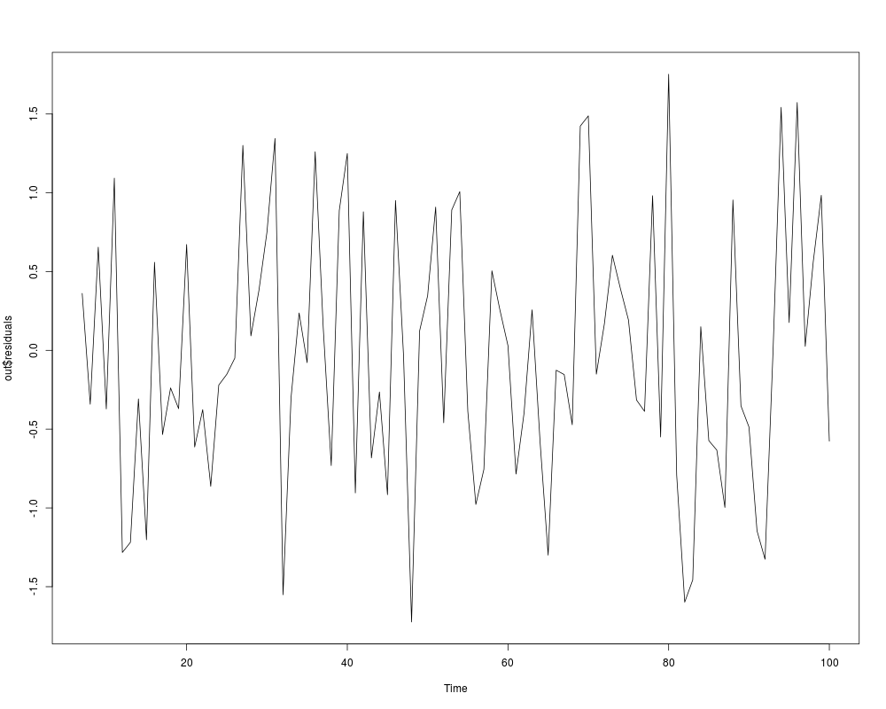
> plot(out$residuals)
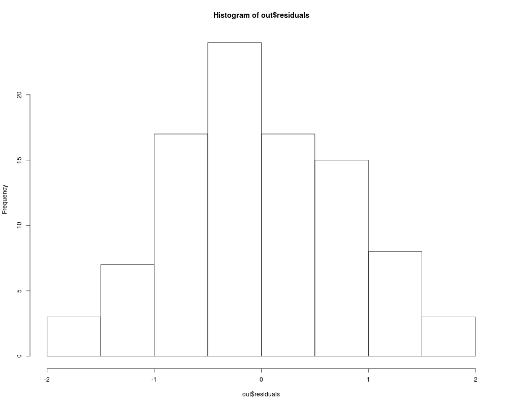
> hist(out$residuals)
> 
> 
> 
> 
> 
> 
> dev.off()
null device 
          1 
>