Supported by Dr. Osamu Ogasawara and  . . |
|
Last data update: 2014.03.03 |
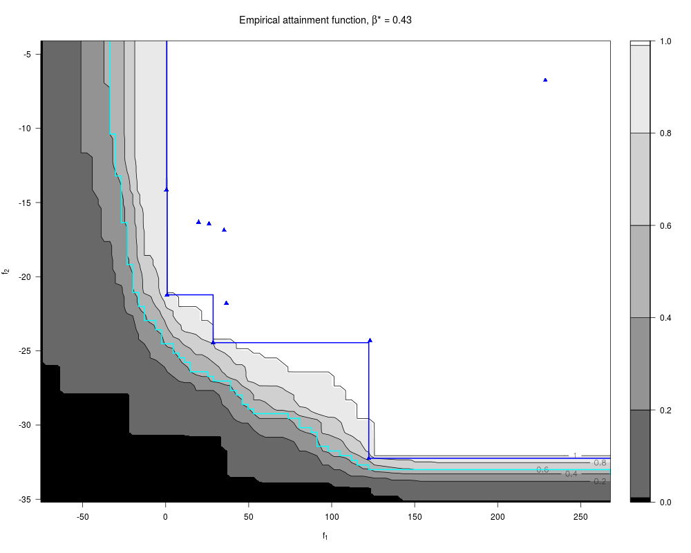
Conditional Pareto Front simulationsDescriptionCompute (on a regular grid) the empirical attainment function from conditional simulations of Gaussian processes corresponding to two objectives. This is used to estimate the Vorob'ev expectation of the attained set and the Vorob'ev deviation. UsageCPF(fun1sims, fun2sims, response, paretoFront = NULL, f1lim = NULL, f2lim = NULL, refPoint = NULL, n.grid = 100, compute.VorobExp = TRUE, compute.VorobDev = TRUE) Arguments
DetailsWorks with two objectives. The user can provide locations of grid lines for
computation of the attainement function with vectors ValueA list which is given the S3 class "
ReferencesM. Binois, D. Ginsbourger and O. Roustant (2015), Quantifying Uncertainty on Pareto Fronts with Gaussian process conditional simulations,
European Journal of Operational Research, 243(2), 386-394. See AlsoMethods Examples
library(DiceDesign)
set.seed(42)

nvar <- 2

fname <- "P1" # Test function

# Initial design
nappr <- 10
design.grid <- maximinESE_LHS(lhsDesign(nappr, nvar, seed = 42)$design)$design
response.grid <- t(apply(design.grid, 1, fname))

# kriging models: matern5_2 covariance structure, linear trend, no nugget effect
mf1 <- km(~., design = design.grid, response = response.grid[,1])
mf2 <- km(~., design = design.grid, response = response.grid[,2])

# Conditional simulations generation with random sampling points
nsim <- 40
npointssim <- 150 # increase for better results
Simu_f1 <- matrix(0, nrow = nsim, ncol = npointssim)
Simu_f2 <- matrix(0, nrow = nsim, ncol = npointssim)
design.sim <- array(0, dim = c(npointssim, nvar, nsim))

for(i in 1:nsim){
  design.sim[,,i] <- matrix(runif(nvar*npointssim), nrow = npointssim, ncol = nvar)
  Simu_f1[i,] <- simulate(mf1, nsim = 1, newdata = design.sim[,,i], cond = TRUE,
                          checkNames = FALSE, nugget.sim = 10^-8)
  Simu_f2[i,] <- simulate(mf2, nsim = 1, newdata = design.sim[,,i], cond = TRUE,
                          checkNames = FALSE, nugget.sim = 10^-8)
}

# Attainment and Voreb'ev expectation + deviation estimation
CPF1 <- CPF(Simu_f1, Simu_f2, response.grid)

# Details about the Vorob'ev threshold  and Vorob'ev deviation
summary(CPF1)

# Graphics
plot(CPF1)
Results
R version 3.3.1 (2016-06-21) -- "Bug in Your Hair"
Copyright (C) 2016 The R Foundation for Statistical Computing
Platform: x86_64-pc-linux-gnu (64-bit)

R is free software and comes with ABSOLUTELY NO WARRANTY.
You are welcome to redistribute it under certain conditions.
Type 'license()' or 'licence()' for distribution details.

R is a collaborative project with many contributors.
Type 'contributors()' for more information and
'citation()' on how to cite R or R packages in publications.

Type 'demo()' for some demos, 'help()' for on-line help, or
'help.start()' for an HTML browser interface to help.
Type 'q()' to quit R.

> library(GPareto)
Loading required package: DiceKriging
Loading required package: emoa
> png(filename="/home/ddbj/snapshot/RGM3/R_CC/result/GPareto/CPF.Rd_%03d_medium.png", width=480, height=480)
> ### Name: CPF
> ### Title: Conditional Pareto Front simulations
> ### Aliases: CPF
>
> ### ** Examples
>
> library(DiceDesign)
> set.seed(42)
>
> nvar <- 2
>
> fname <- "P1" # Test function
>
> # Initial design
> nappr <- 10
> design.grid <- maximinESE_LHS(lhsDesign(nappr, nvar, seed = 42)$design)$design
> response.grid <- t(apply(design.grid, 1, fname))
>
> # kriging models: matern5_2 covariance structure, linear trend, no nugget effect
> mf1 <- km(~., design = design.grid, response = response.grid[,1])

optimisation start
------------------
* estimation method   : MLE
* optimisation method : BFGS
* analytical gradient : used
* trend model : ~X1 + X2
* covariance model :
  - type :  matern5_2
  - nugget : NO
  - parameters lower bounds :  1e-10 1e-10
  - parameters upper bounds :  1.745388 1.748636
  - best initial criterion value(s) :  -55.52774

N = 2, M = 5 machine precision = 2.22045e-16
At X0, 0 variables are exactly at the bounds
At iterate     0  f=       55.528  |proj g|=       1.5181
At iterate     1  f =       55.339  |proj g|=         1.182
At iterate     2  f =       55.296  |proj g|=       0.82441
At iterate     3  f =       55.279  |proj g|=        0.2453
At iterate     4  f =       55.277  |proj g|=      0.022382
At iterate     5  f =       55.277  |proj g|=    0.00072791
At iterate     6  f =       55.277  |proj g|=    2.2922e-06

iterations 6
function evaluations 9
segments explored during Cauchy searches 7
BFGS updates skipped 0
active bounds at final generalized Cauchy point 0
norm of the final projected gradient 2.29218e-06
final function value 55.2772

F = 55.2772
final  value 55.277236
converged
> mf2 <- km(~., design = design.grid, response = response.grid[,2])

optimisation start
------------------
* estimation method   : MLE
* optimisation method : BFGS
* analytical gradient : used
* trend model : ~X1 + X2
* covariance model :
  - type :  matern5_2
  - nugget : NO
  - parameters lower bounds :  1e-10 1e-10
  - parameters upper bounds :  1.745388 1.748636
  - best initial criterion value(s) :  -23.96706

N = 2, M = 5 machine precision = 2.22045e-16
At X0, 0 variables are exactly at the bounds
At iterate     0  f=       23.967  |proj g|=      0.62116
At iterate     1  f =       23.871  |proj g|=       0.17494
At iterate     2  f =       23.864  |proj g|=       0.06536
At iterate     3  f =       23.864  |proj g|=      0.056871
At iterate     4  f =       23.864  |proj g|=      0.016457
At iterate     5  f =       23.864  |proj g|=     0.0086264
At iterate     6  f =       23.864  |proj g|=    2.4015e-05
At iterate     7  f =       23.864  |proj g|=    6.6424e-07

iterations 7
function evaluations 9
segments explored during Cauchy searches 8
BFGS updates skipped 0
active bounds at final generalized Cauchy point 0
norm of the final projected gradient 6.64242e-07
final function value 23.8636

F = 23.8636
final  value 23.863564
converged
>
> # Conditional simulations generation with random sampling points
> nsim <- 40
> npointssim <- 150 # increase for better results
> Simu_f1 <- matrix(0, nrow = nsim, ncol = npointssim)
> Simu_f2 <- matrix(0, nrow = nsim, ncol = npointssim)
> design.sim <- array(0, dim = c(npointssim, nvar, nsim))
>
> for(i in 1:nsim){
+   design.sim[,,i] <- matrix(runif(nvar*npointssim), nrow = npointssim, ncol = nvar)
+   Simu_f1[i,] <- simulate(mf1, nsim = 1, newdata = design.sim[,,i], cond = TRUE,
+                           checkNames = FALSE, nugget.sim = 10^-8)
+   Simu_f2[i,] <- simulate(mf2, nsim = 1, newdata = design.sim[,,i], cond = TRUE,
+                           checkNames = FALSE, nugget.sim = 10^-8)
+ }
>
> # Attainment and Voreb'ev expectation + deviation estimation
> CPF1 <- CPF(Simu_f1, Simu_f2, response.grid)
>
> # Details about the Vorob'ev threshold  and Vorob'ev deviation
> summary(CPF1)

 Number of simulations used: 40

 Number of simulations points: 150

 Ref Point: 267.902 -4.099008

 Ideal Point: -75.22895 -35.20056

 Vorob'ev threshold: 0.425293

 Vorob'ev deviation: 565.0871
>
> # Graphics
> plot(CPF1)
>
>
>
>
>
> dev.off()
null device
          1
>
|