R Graphical Manual

Browse All

Last data update: 2014.03.03

R: Expected Maximin Improvement with m objectives

crit_EMI

R Documentation

Expected Maximin Improvement with m objectives

Description

Expected Maximin Improvement with respect to the current Pareto front with Sample Average Approximation. To avoid numerical instabilities, the new point is penalized if it is too close to an existing observation.

Usage

crit_EMI(x, model, paretoFront = NULL, critcontrol = list(nb.samp = 100,
  seed = 42), type = "UK")

Arguments

`x`	a vector representing the input for which one wishes to calculate `EMI`,
`model`	list of objects of class `km`, one for each objective functions,
`paretoFront`	(optional) matrix corresponding to the Pareto front of size `[n.pareto x n.obj]`,
`critcontrol`	optional list with arguments: `nb.samp` number of random samples from the posterior distribution, default to `50`, increasing gives more reliable results at the cost of longer computation time; `seed` seed used for the random samples. Options for the `checkPredict` function: `threshold` (`1e-4`) and `distance` (`covdist`) are used to avoid numerical issues occuring when adding points too close to the existing ones.
`type`	"`SK`" or "`UK`" (by default), depending whether uncertainty related to trend estimation has to be taken into account.

Details

It is recommanded to scale objectives, e.g. to [0,1].

Value

The Expected Maximin Improvement at x.

References

J. D. Svenson & T. J. Santner (2010), Multiobjective Optimization of Expensive Black-Box Functions via Expected Maximin Improvement, Technical Report.

J. D. Svenson (2011), Computer Experiments: Multiobjective Optimization and Sensitivity Analysis, Ohio State University, PhD thesis.

Examples

#---------------------------------------------------------------------------
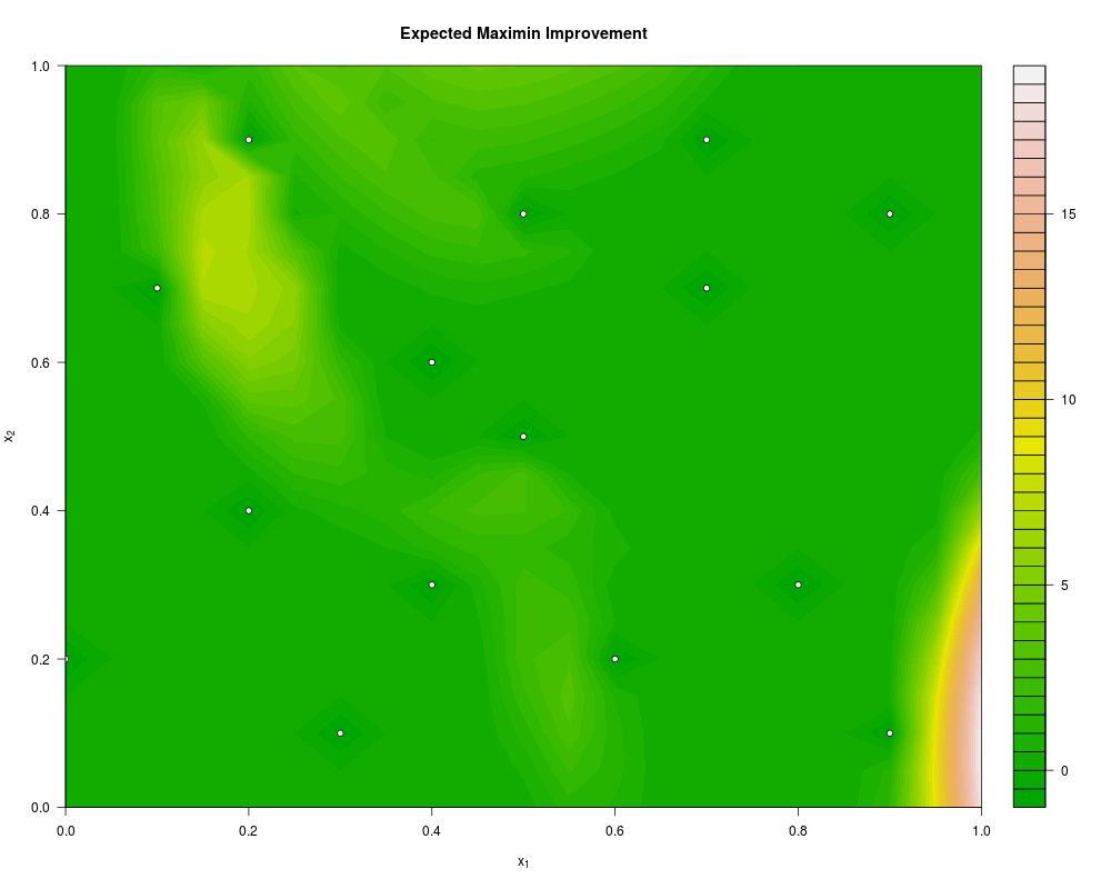
# Expected Maximin Improvement surface associated with the "P1" problem at a 15 points design
#---------------------------------------------------------------------------
set.seed(25468)
library(DiceDesign)

n_var <- 2
f_name <- "P1"
n.grid <- 21
test.grid <- expand.grid(seq(0, 1, length.out = n.grid), seq(0, 1, length.out = n.grid))
n_appr <- 15
design.grid <- round(maximinESE_LHS(lhsDesign(n_appr, n_var, seed = 42)$design)$design, 1)
response.grid <- t(apply(design.grid, 1, f_name))
Front_Pareto <- t(nondominated_points(t(response.grid)))
mf1 <- km(~., design = design.grid, response = response.grid[,1])
mf2 <- km(~., design = design.grid, response = response.grid[,2])

EMI_grid <- apply(test.grid, 1, crit_EMI, model = list(mf1, mf2),
                     critcontrol = list(nb_samp = 20))

filled.contour(seq(0, 1, length.out = n.grid), seq(0, 1, length.out = n.grid), nlevels = 50,
               matrix(EMI_grid, nrow = n.grid), main = "Expected Maximin Improvement",
               xlab = expression(x[1]), ylab = expression(x[2]), color = terrain.colors,
               plot.axes = {axis(1); axis(2);
                            points(design.grid[,1], design.grid[,2], pch = 21, bg = "white")
                            }
              )

Results


R version 3.3.1 (2016-06-21) -- "Bug in Your Hair"
Copyright (C) 2016 The R Foundation for Statistical Computing
Platform: x86_64-pc-linux-gnu (64-bit)

R is free software and comes with ABSOLUTELY NO WARRANTY.
You are welcome to redistribute it under certain conditions.
Type 'license()' or 'licence()' for distribution details.

R is a collaborative project with many contributors.
Type 'contributors()' for more information and
'citation()' on how to cite R or R packages in publications.

Type 'demo()' for some demos, 'help()' for on-line help, or
'help.start()' for an HTML browser interface to help.
Type 'q()' to quit R.

> library(GPareto)
Loading required package: DiceKriging
Loading required package: emoa
> png(filename="/home/ddbj/snapshot/RGM3/R_CC/result/GPareto/crit_EMI.Rd_%03d_medium.png", width=480, height=480)
> ### Name: crit_EMI
> ### Title: Expected Maximin Improvement with m objectives
> ### Aliases: crit_EMI
> 
> ### ** Examples
> 
> #---------------------------------------------------------------------------
> # Expected Maximin Improvement surface associated with the "P1" problem at a 15 points design
> #---------------------------------------------------------------------------
> set.seed(25468)
> library(DiceDesign)
> 
> n_var <- 2
> f_name <- "P1"
> n.grid <- 21
> test.grid <- expand.grid(seq(0, 1, length.out = n.grid), seq(0, 1, length.out = n.grid))
> n_appr <- 15
> design.grid <- round(maximinESE_LHS(lhsDesign(n_appr, n_var, seed = 42)$design)$design, 1)
> response.grid <- t(apply(design.grid, 1, f_name))
> Front_Pareto <- t(nondominated_points(t(response.grid)))
> mf1 <- km(~., design = design.grid, response = response.grid[,1])

optimisation start
------------------
* estimation method   : MLE 
* optimisation method : BFGS 
* analytical gradient : used
* trend model : ~X1 + X2
* covariance model : 
  - type :  matern5_2 
  - nugget : NO
  - parameters lower bounds :  1e-10 1e-10 
  - parameters upper bounds :  1.8 1.6 
  - best initial criterion value(s) :  -76.65715 

N = 2, M = 5 machine precision = 2.22045e-16
At X0, 0 variables are exactly at the bounds
At iterate     0  f=       76.657  |proj g|=      0.56548
At iterate     1  f =       76.655  |proj g|=       0.34575
At iterate     2  f =       76.654  |proj g|=       0.12388
At iterate     3  f =       76.653  |proj g|=       0.18386
At iterate     4  f =        76.65  |proj g|=       0.33277
At iterate     5  f =       76.646  |proj g|=       0.27654
At iterate     6  f =       76.645  |proj g|=      0.036836
At iterate     7  f =       76.645  |proj g|=     0.0004571
At iterate     8  f =       76.645  |proj g|=    8.0283e-06

iterations 8
function evaluations 11
segments explored during Cauchy searches 9
BFGS updates skipped 0
active bounds at final generalized Cauchy point 0
norm of the final projected gradient 8.0283e-06
final function value 76.645

F = 76.645
final  value 76.644956 
converged
> mf2 <- km(~., design = design.grid, response = response.grid[,2])

optimisation start
------------------
* estimation method   : MLE 
* optimisation method : BFGS 
* analytical gradient : used
* trend model : ~X1 + X2
* covariance model : 
  - type :  matern5_2 
  - nugget : NO
  - parameters lower bounds :  1e-10 1e-10 
  - parameters upper bounds :  1.8 1.6 
  - best initial criterion value(s) :  -33.3348 

N = 2, M = 5 machine precision = 2.22045e-16
At X0, 0 variables are exactly at the bounds
At iterate     0  f=       33.335  |proj g|=      0.68325
At iterate     1  f =        32.47  |proj g|=       0.58269
At iterate     2  f =       31.455  |proj g|=       0.30827
At iterate     3  f =       31.408  |proj g|=       0.28827
At iterate     4  f =       31.379  |proj g|=       0.16898
At iterate     5  f =       31.378  |proj g|=       0.13107
At iterate     6  f =       31.377  |proj g|=       0.14969
At iterate     7  f =       31.376  |proj g|=       0.12281
At iterate     8  f =       31.376  |proj g|=     0.0048466
At iterate     9  f =       31.376  |proj g|=    7.7591e-05
At iterate    10  f =       31.376  |proj g|=    6.0651e-08

iterations 10
function evaluations 14
segments explored during Cauchy searches 11
BFGS updates skipped 0
active bounds at final generalized Cauchy point 0
norm of the final projected gradient 6.06512e-08
final function value 31.3756

F = 31.3756
final  value 31.375637 
converged
> 
> EMI_grid <- apply(test.grid, 1, crit_EMI, model = list(mf1, mf2),
+                      critcontrol = list(nb_samp = 20))
> 
> filled.contour(seq(0, 1, length.out = n.grid), seq(0, 1, length.out = n.grid), nlevels = 50,
+                matrix(EMI_grid, nrow = n.grid), main = "Expected Maximin Improvement",
+                xlab = expression(x[1]), ylab = expression(x[2]), color = terrain.colors,
+                plot.axes = {axis(1); axis(2);
+                             points(design.grid[,1], design.grid[,2], pch = 21, bg = "white")
+                             }
+               )
> 
> 
> 
> 
> 
> dev.off()
null device 
          1 
>