R Graphical Manual

Browse All

Last data update: 2014.03.03

R: Analytical expression of the SMS-EGO criterion with m>1...

crit_SMS

R Documentation

Analytical expression of the SMS-EGO criterion with m>1 objectives

Description

Computes a slightly modified infill Criterion of the SMS-EGO. To avoid numerical instabilities, an additional penalty is added to the new point if it is too close to an existing observation.

Usage

crit_SMS(x, model, paretoFront = NULL, critcontrol = list(epsilon = 1e-06,
  gain = 1), type = "UK")

Arguments

`x`	a vector representing the input for which one wishes to calculate the criterion,
`model`	a list of objects of class `km` (one for each objective),
`paretoFront`	(optional) matrix corresponding to the Pareto front of size `[n.pareto x n.obj]`,
`critcontrol`	list with arguments: `currentHV` current hypervolume; `refPoint` reference point for hypervolume computations; `epsilon` optional value to use in additive epsilon dominance; `gain` optional gain factor for sigma. Options for the `checkPredict` function: `threshold` (`1e-4`) and `distance` (`covdist`) are used to avoid numerical issues occuring when adding points too close to the existing ones.
`type`	"`SK`" or "`UK`" (by default), depending whether uncertainty related to trend estimation has to be taken into account.

Value

Value of the criterion.

References

W. Ponweiser, T. Wagner, D. Biermann, M. Vincze (2008), Multiobjective Optimization on a Limited Budget of Evaluations Using Model-Assisted S-Metric Selection, Parallel Problem Solving from Nature, pp. 784-794. Springer, Berlin.

T. Wagner, M. Emmerich, A. Deutz, W. Ponweiser (2010), On expected-improvement criteria for model-based multi-objective optimization. Parallel Problem Solving from Nature, pp. 718-727. Springer, Berlin.

Examples

#---------------------------------------------------------------------------
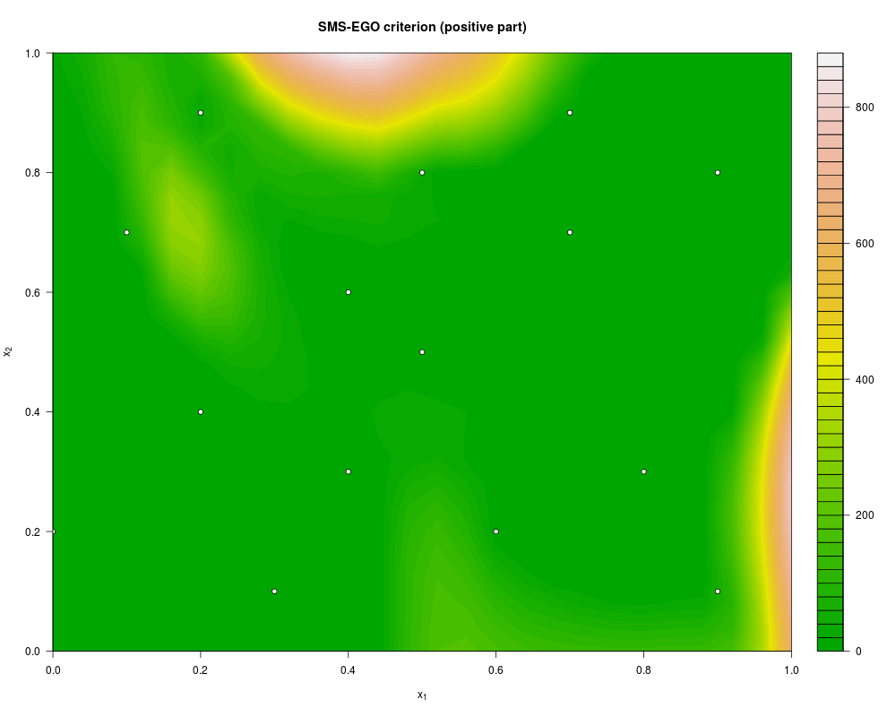
# SMS-EGO surface associated with the "P1" problem at a 15 points design
#---------------------------------------------------------------------------
set.seed(25468)
library(DiceDesign)

n_var <- 2
f_name <- "P1"
n.grid <- 26
test.grid <- expand.grid(seq(0, 1, length.out = n.grid), seq(0, 1, length.out = n.grid))
n_appr <- 15
design.grid <- round(maximinESE_LHS(lhsDesign(n_appr, n_var, seed = 42)$design)$design, 1)
response.grid <- t(apply(design.grid, 1, f_name))
PF <- t(nondominated_points(t(response.grid)))
mf1 <- km(~., design = design.grid, response = response.grid[,1])
mf2 <- km(~., design = design.grid, response = response.grid[,2])

model <- list(mf1, mf2)
critcontrol <- list(refPoint = c(300, 0), currentHV = dominated_hypervolume(t(PF), c(300, 0)))
SMSEGO_grid <- apply(test.grid, 1, crit_SMS, model = model,
                     paretoFront = PF, critcontrol = critcontrol)

filled.contour(seq(0, 1, length.out = n.grid), seq(0, 1, length.out = n.grid),
               matrix(pmax(0, SMSEGO_grid), nrow = n.grid), nlevels = 50,
               main = "SMS-EGO criterion (positive part)", xlab = expression(x[1]),
               ylab = expression(x[2]), color = terrain.colors,
               plot.axes = {axis(1); axis(2);
                            points(design.grid[,1],design.grid[,2], pch = 21, bg = "white")
                            }
              )

Results


R version 3.3.1 (2016-06-21) -- "Bug in Your Hair"
Copyright (C) 2016 The R Foundation for Statistical Computing
Platform: x86_64-pc-linux-gnu (64-bit)

R is free software and comes with ABSOLUTELY NO WARRANTY.
You are welcome to redistribute it under certain conditions.
Type 'license()' or 'licence()' for distribution details.

R is a collaborative project with many contributors.
Type 'contributors()' for more information and
'citation()' on how to cite R or R packages in publications.

Type 'demo()' for some demos, 'help()' for on-line help, or
'help.start()' for an HTML browser interface to help.
Type 'q()' to quit R.

> library(GPareto)
Loading required package: DiceKriging
Loading required package: emoa
> png(filename="/home/ddbj/snapshot/RGM3/R_CC/result/GPareto/crit_SMS.Rd_%03d_medium.png", width=480, height=480)
> ### Name: crit_SMS
> ### Title: Analytical expression of the SMS-EGO criterion with m>1
> ###   objectives
> ### Aliases: crit_SMS
> 
> ### ** Examples
> 
> #---------------------------------------------------------------------------
> # SMS-EGO surface associated with the "P1" problem at a 15 points design
> #---------------------------------------------------------------------------
> set.seed(25468)
> library(DiceDesign)
> 
> n_var <- 2
> f_name <- "P1"
> n.grid <- 26
> test.grid <- expand.grid(seq(0, 1, length.out = n.grid), seq(0, 1, length.out = n.grid))
> n_appr <- 15
> design.grid <- round(maximinESE_LHS(lhsDesign(n_appr, n_var, seed = 42)$design)$design, 1)
> response.grid <- t(apply(design.grid, 1, f_name))
> PF <- t(nondominated_points(t(response.grid)))
> mf1 <- km(~., design = design.grid, response = response.grid[,1])

optimisation start
------------------
* estimation method   : MLE 
* optimisation method : BFGS 
* analytical gradient : used
* trend model : ~X1 + X2
* covariance model : 
  - type :  matern5_2 
  - nugget : NO
  - parameters lower bounds :  1e-10 1e-10 
  - parameters upper bounds :  1.8 1.6 
  - best initial criterion value(s) :  -76.65715 

N = 2, M = 5 machine precision = 2.22045e-16
At X0, 0 variables are exactly at the bounds
At iterate     0  f=       76.657  |proj g|=      0.56548
At iterate     1  f =       76.655  |proj g|=       0.34575
At iterate     2  f =       76.654  |proj g|=       0.12388
At iterate     3  f =       76.653  |proj g|=       0.18386
At iterate     4  f =        76.65  |proj g|=       0.33277
At iterate     5  f =       76.646  |proj g|=       0.27654
At iterate     6  f =       76.645  |proj g|=      0.036836
At iterate     7  f =       76.645  |proj g|=     0.0004571
At iterate     8  f =       76.645  |proj g|=    8.0283e-06

iterations 8
function evaluations 11
segments explored during Cauchy searches 9
BFGS updates skipped 0
active bounds at final generalized Cauchy point 0
norm of the final projected gradient 8.0283e-06
final function value 76.645

F = 76.645
final  value 76.644956 
converged
> mf2 <- km(~., design = design.grid, response = response.grid[,2])

optimisation start
------------------
* estimation method   : MLE 
* optimisation method : BFGS 
* analytical gradient : used
* trend model : ~X1 + X2
* covariance model : 
  - type :  matern5_2 
  - nugget : NO
  - parameters lower bounds :  1e-10 1e-10 
  - parameters upper bounds :  1.8 1.6 
  - best initial criterion value(s) :  -33.3348 

N = 2, M = 5 machine precision = 2.22045e-16
At X0, 0 variables are exactly at the bounds
At iterate     0  f=       33.335  |proj g|=      0.68325
At iterate     1  f =        32.47  |proj g|=       0.58269
At iterate     2  f =       31.455  |proj g|=       0.30827
At iterate     3  f =       31.408  |proj g|=       0.28827
At iterate     4  f =       31.379  |proj g|=       0.16898
At iterate     5  f =       31.378  |proj g|=       0.13107
At iterate     6  f =       31.377  |proj g|=       0.14969
At iterate     7  f =       31.376  |proj g|=       0.12281
At iterate     8  f =       31.376  |proj g|=     0.0048466
At iterate     9  f =       31.376  |proj g|=    7.7591e-05
At iterate    10  f =       31.376  |proj g|=    6.0651e-08

iterations 10
function evaluations 14
segments explored during Cauchy searches 11
BFGS updates skipped 0
active bounds at final generalized Cauchy point 0
norm of the final projected gradient 6.06512e-08
final function value 31.3756

F = 31.3756
final  value 31.375637 
converged
> 
> model <- list(mf1, mf2)
> critcontrol <- list(refPoint = c(300, 0), currentHV = dominated_hypervolume(t(PF), c(300, 0)))
> SMSEGO_grid <- apply(test.grid, 1, crit_SMS, model = model,
+                      paretoFront = PF, critcontrol = critcontrol)
> 
> filled.contour(seq(0, 1, length.out = n.grid), seq(0, 1, length.out = n.grid),
+                matrix(pmax(0, SMSEGO_grid), nrow = n.grid), nlevels = 50,
+                main = "SMS-EGO criterion (positive part)", xlab = expression(x[1]),
+                ylab = expression(x[2]), color = terrain.colors,
+                plot.axes = {axis(1); axis(2);
+                             points(design.grid[,1],design.grid[,2], pch = 21, bg = "white")
+                             }
+               )
> 
> 
> 
> 
> 
> dev.off()
null device 
          1 
>