Display the Symmetric Deviation Function

Description

Display the Symmetric Deviation Function for an object of class CPF.

Usage

plotSymDevFun(CPF, n.grid = 100)

Arguments

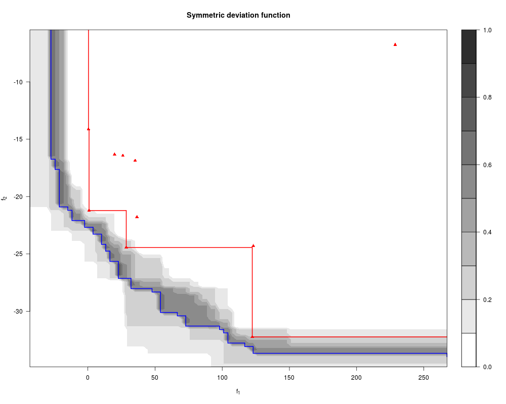
Details

Display observations in red and the corresponding Pareto front by a step-line. The blue line is the estimation of the location of the Pareto front of the kriging models, named Vorob'ev expectation. In grayscale is the intensity of the deviation (symmetrical difference) from the Vorob'ev expectation for couples of conditional simulations.

References

M. Binois, D. Ginsbourger and O. Roustant (2015), Quantifying Uncertainty on Pareto Fronts with Gaussian process conditional simulations, European Journal of Operational Research, 243(2), 386-394.

Examples

library(DiceDesign)
set.seed(42)

nvar <- 2

# Test function
fname = "P1"

# Initial design
nappr <- 10
design.grid <- maximinESE_LHS(lhsDesign(nappr, nvar, seed = 42)$design)$design
response.grid <- t(apply(design.grid, 1, fname))

ParetoFront <- t(nondominated_points(t(response.grid)))

# kriging models : matern5_2 covariance structure, linear trend, no nugget effect
mf1 <- km(~., design = design.grid, response = response.grid[, 1])
mf2 <- km(~., design = design.grid, response = response.grid[, 2])

# Conditional simulations generation with random sampling points
nsim <- 10 # increase for better results
npointssim <- 80 # increase for better results
Simu_f1 = matrix(0, nrow = nsim, ncol = npointssim)
Simu_f2 = matrix(0, nrow = nsim, ncol = npointssim)
design.sim = array(0,dim = c(npointssim, nvar, nsim))

for(i in 1:nsim){
  design.sim[,, i] <- matrix(runif(nvar*npointssim), npointssim, nvar)
  Simu_f1[i,] = simulate(mf1, nsim = 1, newdata = design.sim[,, i], cond = TRUE,
                         checkNames = FALSE, nugget.sim = 10^-8)
  Simu_f2[i,] = simulate(mf2, nsim = 1, newdata = design.sim[,, i], cond=TRUE,
                         checkNames = FALSE, nugget.sim = 10^-8)
}

# Attainment, Voreb'ev expectation and deviation estimation
CPF1 <- CPF(Simu_f1, Simu_f2, response.grid, ParetoFront)

# Symmetric deviation function
plotSymDevFun(CPF1)

Results

R version 3.3.1 (2016-06-21) -- "Bug in Your Hair"
Copyright (C) 2016 The R Foundation for Statistical Computing
Platform: x86_64-pc-linux-gnu (64-bit)

R is free software and comes with ABSOLUTELY NO WARRANTY.
You are welcome to redistribute it under certain conditions.
Type 'license()' or 'licence()' for distribution details.

R is a collaborative project with many contributors.
Type 'contributors()' for more information and
'citation()' on how to cite R or R packages in publications.

Type 'demo()' for some demos, 'help()' for on-line help, or
'help.start()' for an HTML browser interface to help.
Type 'q()' to quit R.

> library(GPareto)
Loading required package: DiceKriging
Loading required package: emoa
> png(filename="/home/ddbj/snapshot/RGM3/R_CC/result/GPareto/plotSymDevFun.Rd_%03d_medium.png", width=480, height=480)
> ### Name: plotSymDevFun
> ### Title: Display the Symmetric Deviation Function
> ### Aliases: plotSymDevFun
> 
> ### ** Examples
> 
> library(DiceDesign)
> set.seed(42)
> 
> nvar <- 2
> 
> # Test function
> fname = "P1"
> 
> # Initial design
> nappr <- 10
> design.grid <- maximinESE_LHS(lhsDesign(nappr, nvar, seed = 42)$design)$design
> response.grid <- t(apply(design.grid, 1, fname))
> 
> ParetoFront <- t(nondominated_points(t(response.grid)))
> 
> # kriging models : matern5_2 covariance structure, linear trend, no nugget effect
> mf1 <- km(~., design = design.grid, response = response.grid[, 1])

optimisation start
------------------
* estimation method   : MLE 
* optimisation method : BFGS 
* analytical gradient : used
* trend model : ~X1 + X2
* covariance model : 
  - type :  matern5_2 
  - nugget : NO
  - parameters lower bounds :  1e-10 1e-10 
  - parameters upper bounds :  1.745388 1.748636 
  - best initial criterion value(s) :  -55.52774 

N = 2, M = 5 machine precision = 2.22045e-16
At X0, 0 variables are exactly at the bounds
At iterate     0  f=       55.528  |proj g|=       1.5181
At iterate     1  f =       55.339  |proj g|=         1.182
At iterate     2  f =       55.296  |proj g|=       0.82441
At iterate     3  f =       55.279  |proj g|=        0.2453
At iterate     4  f =       55.277  |proj g|=      0.022382
At iterate     5  f =       55.277  |proj g|=    0.00072791
At iterate     6  f =       55.277  |proj g|=    2.2922e-06

iterations 6
function evaluations 9
segments explored during Cauchy searches 7
BFGS updates skipped 0
active bounds at final generalized Cauchy point 0
norm of the final projected gradient 2.29218e-06
final function value 55.2772

F = 55.2772
final  value 55.277236 
converged
> mf2 <- km(~., design = design.grid, response = response.grid[, 2])

optimisation start
------------------
* estimation method   : MLE 
* optimisation method : BFGS 
* analytical gradient : used
* trend model : ~X1 + X2
* covariance model : 
  - type :  matern5_2 
  - nugget : NO
  - parameters lower bounds :  1e-10 1e-10 
  - parameters upper bounds :  1.745388 1.748636 
  - best initial criterion value(s) :  -23.96706 

N = 2, M = 5 machine precision = 2.22045e-16
At X0, 0 variables are exactly at the bounds
At iterate     0  f=       23.967  |proj g|=      0.62116
At iterate     1  f =       23.871  |proj g|=       0.17494
At iterate     2  f =       23.864  |proj g|=       0.06536
At iterate     3  f =       23.864  |proj g|=      0.056871
At iterate     4  f =       23.864  |proj g|=      0.016457
At iterate     5  f =       23.864  |proj g|=     0.0086264
At iterate     6  f =       23.864  |proj g|=    2.4015e-05
At iterate     7  f =       23.864  |proj g|=    6.6424e-07

iterations 7
function evaluations 9
segments explored during Cauchy searches 8
BFGS updates skipped 0
active bounds at final generalized Cauchy point 0
norm of the final projected gradient 6.64242e-07
final function value 23.8636

F = 23.8636
final  value 23.863564 
converged
> 
> # Conditional simulations generation with random sampling points
> nsim <- 10 # increase for better results
> npointssim <- 80 # increase for better results
> Simu_f1 = matrix(0, nrow = nsim, ncol = npointssim)
> Simu_f2 = matrix(0, nrow = nsim, ncol = npointssim)
> design.sim = array(0,dim = c(npointssim, nvar, nsim))
> 
> for(i in 1:nsim){
+   design.sim[,, i] <- matrix(runif(nvar*npointssim), npointssim, nvar)
+   Simu_f1[i,] = simulate(mf1, nsim = 1, newdata = design.sim[,, i], cond = TRUE,
+                          checkNames = FALSE, nugget.sim = 10^-8)
+   Simu_f2[i,] = simulate(mf2, nsim = 1, newdata = design.sim[,, i], cond=TRUE,
+                          checkNames = FALSE, nugget.sim = 10^-8)
+ }
> 
> # Attainment, Voreb'ev expectation and deviation estimation
> CPF1 <- CPF(Simu_f1, Simu_f2, response.grid, ParetoFront)
> 
> # Symmetric deviation function
> plotSymDevFun(CPF1)
> 
> 
> 
> 
> 
> dev.off()
null device 
          1 
>