Supported by Dr. Osamu Ogasawara and  . . |
|
Last data update: 2014.03.03 |
Plotting GP model fitsDescriptionPlots the predicted response and mean squared error (MSE) surfaces for simulators with 1 and 2 dimensional inputs (i.e. d = 1,2). Usage
## S3 method for class 'GP'
plot(x, M = 1, range = c(0, 1), resolution = 50,
colors = c('black', 'blue', 'red'), line_type = c(1, 2),
pch = 20, cex = 1, legends = FALSE, surf_check = FALSE,
response = TRUE, ...)
Arguments
For 1 Dimensional Plotting
Author(s)Blake MacDonald, Hugh Chipman, Pritam Ranjan ReferencesRanjan, P., Haynes, R., and Karsten, R. (2011). A Computationally Stable Approach to Gaussian Process Interpolation of Deterministic Computer Simulation Data, Technometrics, 53(4), 366 - 378. See Also
Examples
## 1D Example 1
n = 5; d = 1;
computer_simulator <- function(x){
x = 2*x+0.5;
y = sin(10*pi*x)/(2*x) + (x-1)^4;
return(y)
}
set.seed(3);
library(lhs);
x = maximinLHS(n,d);
y = computer_simulator(x);
GPmodel = GP_fit(x,y);
plot.GP(GPmodel)
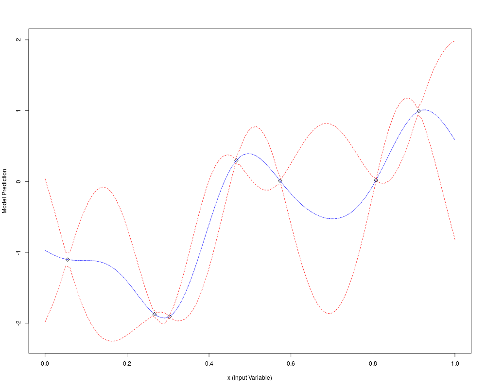
## 1D Example 2
n = 7; d = 1;
computer_simulator <- function(x) {
y = log(x+0.1)+sin(5*pi*x);
return(y)
}
set.seed(1);
library(lhs);
x = maximinLHS(n,d);
y = computer_simulator(x);
GPmodel = GP_fit(x,y);
## Plotting with changes from the default line type and characters
plot.GP(GPmodel, resolution = 100, line_type = c(6,2), pch = 5)
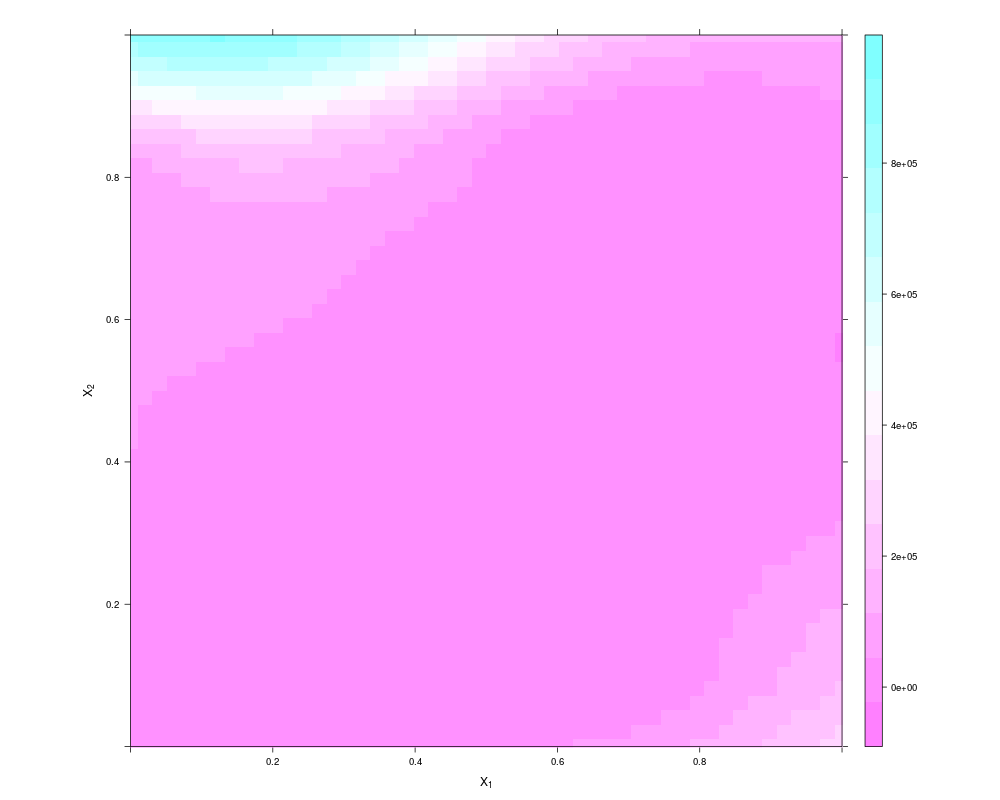
## 2D Example: GoldPrice Function
computer_simulator <- function(x) {
x1=4*x[,1] - 2; x2=4*x[,2] - 2;
t1 = 1 + (x1 + x2 + 1)^2*(19 - 14*x1 + 3*x1^2 - 14*x2 +
6*x1*x2 + 3*x2^2);
t2 = 30 + (2*x1 -3*x2)^2*(18 - 32*x1 + 12*x1^2 + 48*x2 -
36*x1*x2 + 27*x2^2);
y = t1*t2;
return(y)
}
n = 30; d = 2;
set.seed(1);
library(lhs);
library(lattice);
x = maximinLHS(n,d);
y = computer_simulator(x);
GPmodel = GP_fit(x,y);
## Basic level plot
plot.GP(GPmodel)
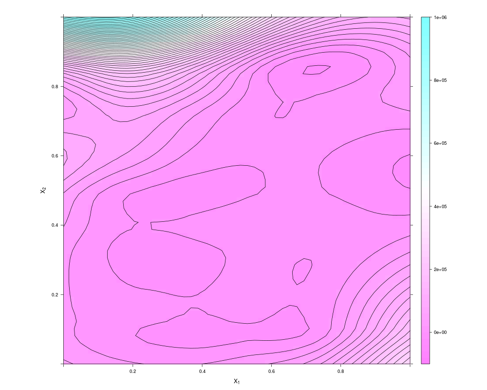
## Adding Contours and increasing the number of levels
plot.GP(GPmodel, contour = TRUE, cuts = 50, pretty = TRUE)
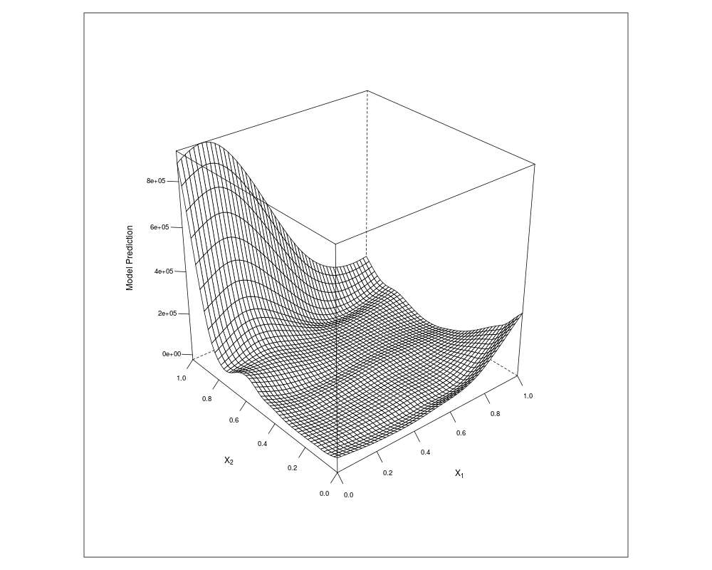
## Plotting the Response Surface
plot.GP(GPmodel, surf_check = TRUE)
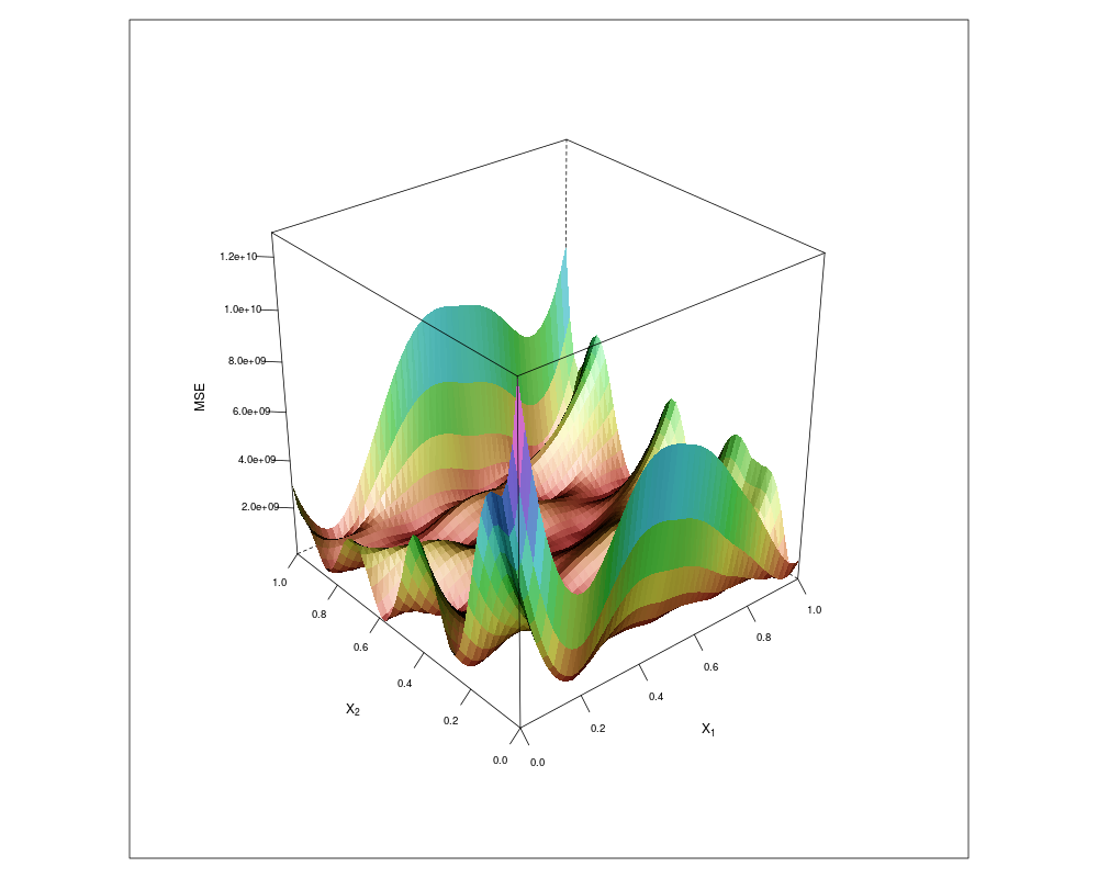
## Plotting the Error Surface with color
plot.GP(GPmodel, surf_check = TRUE, response = FALSE, shade = TRUE)
Results
R version 3.3.1 (2016-06-21) -- "Bug in Your Hair"
Copyright (C) 2016 The R Foundation for Statistical Computing
Platform: x86_64-pc-linux-gnu (64-bit)

R is free software and comes with ABSOLUTELY NO WARRANTY.
You are welcome to redistribute it under certain conditions.
Type 'license()' or 'licence()' for distribution details.

R is a collaborative project with many contributors.
Type 'contributors()' for more information and
'citation()' on how to cite R or R packages in publications.

Type 'demo()' for some demos, 'help()' for on-line help, or
'help.start()' for an HTML browser interface to help.
Type 'q()' to quit R.

> library(GPfit)
> png(filename="/home/ddbj/snapshot/RGM3/R_CC/result/GPfit/plot.GP.Rd_%03d_medium.png", width=480, height=480)
> ### Name: plot.GP
> ### Title: Plotting GP model fits
> ### Aliases: plot.GP
>
> ### ** Examples
>
> ## 1D Example 1
> n = 5; d = 1;
> computer_simulator <- function(x){
+ x = 2*x+0.5;
+ y = sin(10*pi*x)/(2*x) + (x-1)^4;
+ return(y)
+ }
> set.seed(3);
> library(lhs);
> x = maximinLHS(n,d);
> y = computer_simulator(x);
> GPmodel = GP_fit(x,y);
> plot.GP(GPmodel)
>
>
> ## 1D Example 2
> n = 7; d = 1;
> computer_simulator <- function(x) {
+ y = log(x+0.1)+sin(5*pi*x);
+ return(y)
+ }
> set.seed(1);
> library(lhs);
> x = maximinLHS(n,d);
> y = computer_simulator(x);
> GPmodel = GP_fit(x,y);
> ## Plotting with changes from the default line type and characters
> plot.GP(GPmodel, resolution = 100, line_type = c(6,2), pch = 5)
>
>
> ## 2D Example: GoldPrice Function
> computer_simulator <- function(x) {
+ x1=4*x[,1] - 2; x2=4*x[,2] - 2;
+ t1 = 1 + (x1 + x2 + 1)^2*(19 - 14*x1 + 3*x1^2 - 14*x2 +
+ 6*x1*x2 + 3*x2^2);
+ t2 = 30 + (2*x1 -3*x2)^2*(18 - 32*x1 + 12*x1^2 + 48*x2 -
+ 36*x1*x2 + 27*x2^2);
+ y = t1*t2;
+ return(y)
+ }
> n = 30; d = 2;
> set.seed(1);
> library(lhs);
> library(lattice);
> x = maximinLHS(n,d);
> y = computer_simulator(x);
> GPmodel = GP_fit(x,y);
> ## Basic level plot
> plot.GP(GPmodel)
> ## Adding Contours and increasing the number of levels
> plot.GP(GPmodel, contour = TRUE, cuts = 50, pretty = TRUE)
> ## Plotting the Response Surface
> plot.GP(GPmodel, surf_check = TRUE)
> ## Plotting the Error Surface with color
> plot.GP(GPmodel, surf_check = TRUE, response = FALSE, shade = TRUE)
>
>
>
>
>
> dev.off()
null device
          1
>
|