R Graphical Manual

Browse All

Last data update: 2014.03.03

R: Fitting the Generalized and Variable Persistence Models

GPvam

R Documentation

Fitting the Generalized and Variable Persistence Models

Description

GPvam is used to fit the value-added model developed by Mariano et al. (2010) via ML estimation using an EM algorithm (Karl et al. 2013). Also provides the ability to fit the variable persistence model (Lockwood et al. 2007).

Usage

GPvam(vam_data, fixed_effects = formula(~as.factor(year) + 0), 
   student.side = "R", persistence="GP", max.iter.EM = 1000, tol1 = 1e-07, 
   hessian = FALSE, hes.method = "simple", verbose = TRUE)

Arguments

`vam_data`	a data frame that contains at least a column "y" containing the student scores, a column "student" containing unique student ID's, a column "teacher" containing the teacher ID's, and a column "year" which contains the year (or semester, etc.) of the time period. The "y" and "year" variables needs to be numeric. If other variables are to be included as fixed effects, they should also be included in vam_data. See 'Note' for further discussion.
`fixed_effects`	an object of class `formula` describing the structure of the fixed effects. Categorical variables should be wrapped in an `as.factor` statement.
`student.side`	a character. Choices are "G" or "R". See section 'Details'.
`persistence`	a character. Choices are "GP", "rGP", "VP", "CP", or "ZP". Only "GP" is currently compatible with student.side="G". See section 'Details'.
`max.iter.EM`	the maximum number of EM iterations
`tol1`	convergence tolerance for EM algorithm. The convergence criterion is specified under 'Details'.
`hessian`	logical indicating whether the Hessian of the variance parameters (and persistence parameters for persistence="VP") should be calculated after convergence of the EM algorithm. Standard errors for the fixed and EBLUPs are calculated by default.
`hes.method`	a character string indicating the method of numerical differentiation used to calculate the Hessian of the variance parameters. Options are "simple" or "richardson".
`verbose`	logical. If TRUE, model information will be printed at each iteration.

Details

The design for the random teacher effects according to the generalized persistence model of Mariano et al. (2010) is built into the function. The model includes correlated current- and future-year effects for each teacher. By setting student.side="R", the intra-student correlation is modeled via an unstructured, block-diagonal error covariance matrix, as specified by Mariano et al. (2010). Setting student.side="G" keeps the same teacher structure, but models intra-student correlation via random student effects. This is similar to the model used by McCaffrey and Lockwood (2011), and is appropriate when the testing scale is the same across years. In this case, the error covariance matrix is diagonal, although a separate variance is calcualted for each year. From a computational perspective, the model estimating the R-side student effects has better scalability properties, although the G-side function is faster (Karl et al. 2012).

The persistence option determines the type of persistence effects that are modeled. The generalized persistence model ("GP") is described above. When student.side="R", other models for teacher persistence are available. The reduced GP model ("rGP", Karl et al. 2012) combines each teacher's future year effects from the GP model into a single effect. The variable persistence model ("VP") assumes that teacher effects in future years are multiples of their effect in the current year (Lockwood et al. 2007). The multipliers in the VP model are called persistence parameters, and are estimated. By contrast, the complete ("CP") and zero ("ZP") persistence models fix the persistence parameters at 1 and 0, respectively (Lockwood et al. 2007).

Convergence is declared when (l_k-l_{k-1})/l_k < 1E-07, where l_k is the log-likelihood at iteration k.

The model is estimated via an EM algorithm. For details, see Karl et al. (2012). The model was estimated through Bayesian computation in Mariano et al. (2010).

Note: When student.side="R" is selected, the first few iterations of the EM algorithm will take longer than subsequent iterations. This is a result of the hybrid gradient-ascent/Newton-Raphson method used in the M-step for the R matrix in the first two iterations (Karl et al. 2012).

Program run time and memory requirements: The data file GPvam.benchmark that is included with the package contains runtime and peak memory requirements for different persistence settings, using simulated data sets with different values for number of years, number of teachers per year, and number of students per teacher. These have been multiplied to show the total number of teachers in the data set, as well as the total number of students. With student.side="R", the persistence="GP" model is most sensitive to increases in the size of the data set. With student.side="G", the memory requirements increase exponentially with the number of students and teachers, and that model should not be considered scalable to extremely large data sets.

All of these benchmarks were performed with Hessian=TRUE. Calculation of the Hessian accounts for anywhere from 20% to 75% of those run times. Unless the standard errors of the variance components are needed, leaving Hessian=FALSE will lead to a faster run time with smaller memory requirements.

Value

GPvam returns an object of class GPvam

An object of class GPvam is a list containing the following components:

`loglik`	the maximized log-likelihood at convergence of the EM algorithm
`teach.effects`	a data frame containing the predicted teacher effects and standard errors
`parameters`	a matrix of estimated model parameters and standard errors
`Hessian`	if requested, the Hessian of the variance parameters
`R_i`	(only when `student_side` is set to 'R') a matrix containing the error covariance matrix of a student
`teach.cov`	a list containing the unique blocks of the covariance matrix of teacher effects
`mresid`	a vector of the raw marginal residuals
`cresid`	a vector of the raw conditional residuals
`sresid`	a vector of the scaled conditional residuals
`yhat`	a vector of the predicted values

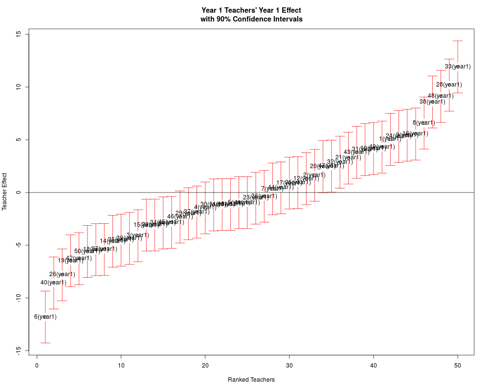
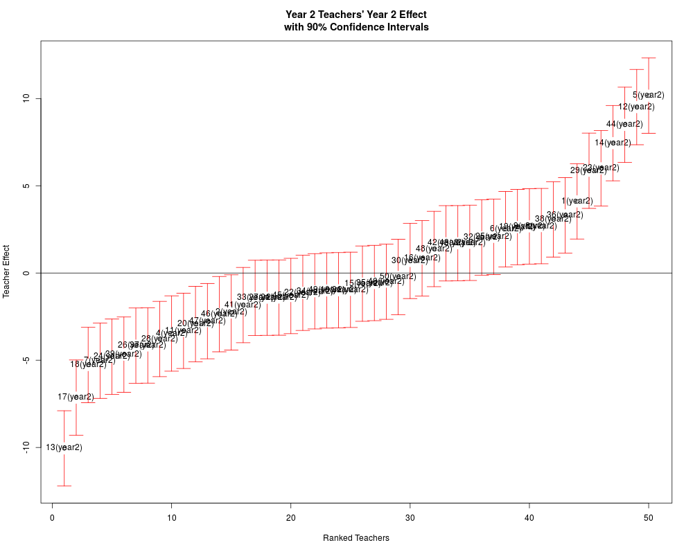
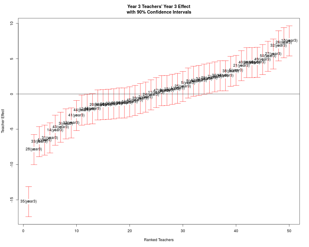
The function summary provides a summary of the results. This includes the estimated model parameters and standard errors, along with the correlation matrices corresponding to the estimated correlation matrices. Summary information about scaled and raw residuals is reported.

Note

The model assumes that each teacher teaches only one year. If, for example, a teacher teaches in years 1 and 2, his/her first year performance is modeled independently of the second year performance. To keep these effects seperate, the progam appends "(year i)" to each teacher name, where i is the year in which the teacher taught.

The fixed_effects argument of GPvam utilizes the functionality of R's formula class. In the statement fixed_effects=formula(~as.factor(year)+cont_var+0)), as.factor(year) identifies year as a categorical variable. +0 indicates that no intercept is to be fitted, and +cont_var indicates that a seperate effect is to be fitted for the continuous variable "cont_var." An interaction between "year" and "cont_var" could be specified by ~as.factor(year)*cont_var+0, or equivalently, ~as.factor(year)+cont_var+as.factor(year):cont_var+0. See formula for more details.

When applied to an object of class GPvam, plot.GPvam returns a caterpillar plot for each effect, as well as residual plots.

Author(s)

Andrew Karl akarl@asu.edu, Yan Yang, Sharon Lohr

References

Karl, A., Yang, Y. and Lohr, S. (2013) Efficient Maximum Likelihood Estimation of Multiple Membership Linear Mixed Models, with an Application to Educational Value-Added Assessments Computational Statistics & Data Analysis 59, 13–27.

Karl, A., Yang, Y. and Lohr, S. (2014) Computation of Maximum Likelihood Estimates for Multiresponse Generalized Linear Mixed Models with Non-nested, Correlated Random Effects Computational Statistics & Data Analysis 73, 146–162.

Karl, A., Yang, Y. and Lohr, S. (2014) A Correlated Random Effects Model for Nonignorable Missing Data in Value-Added Assessment of Teacher Effects Journal of Educational and Behavioral Statistics 38, 577–603.

Lockwood, J., McCaffrey, D., Mariano, L., Setodji, C. (2007) Bayesian Methods for Scalable Multivariate Value-Added Assesment. Journal of Educational and Behavioral Statistics 32, 125–150.

Mariano, L., McCaffrey, D. and Lockwood, J. (2010) A Model for Teacher Effects From Longitudinal Data Without Assuming Vertical Scaling. Journal of Educational and Behavioral Statistics 35, 253–279.

McCaffrey, D. and Lockwood, J. (2011) Missing Data in Value-Added Modeling of Teacher Effects," Annals of Applied Statistics 5, 773–797

Examples

data(vam_data)
GPvam(vam_data,student.side="R",persistence="VP",
fixed_effects=formula(~as.factor(year)+cont_var+0),verbose=TRUE,max.iter.EM=1)

result <- GPvam(vam_data,student.side="R",persistence="VP",
fixed_effects=formula(~as.factor(year)+cont_var+0),verbose=TRUE)
 summary(result)

 plot(result)

Results


R version 3.3.1 (2016-06-21) -- "Bug in Your Hair"
Copyright (C) 2016 The R Foundation for Statistical Computing
Platform: x86_64-pc-linux-gnu (64-bit)

R is free software and comes with ABSOLUTELY NO WARRANTY.
You are welcome to redistribute it under certain conditions.
Type 'license()' or 'licence()' for distribution details.

R is a collaborative project with many contributors.
Type 'contributors()' for more information and
'citation()' on how to cite R or R packages in publications.

Type 'demo()' for some demos, 'help()' for on-line help, or
'help.start()' for an HTML browser interface to help.
Type 'q()' to quit R.

> library(GPvam)
Loading required package: Matrix
> png(filename="/home/ddbj/snapshot/RGM3/R_CC/result/GPvam/GPvam.Rd_%03d_medium.png", width=480, height=480)
> ### Name: GPvam
> ### Title: Fitting the Generalized and Variable Persistence Models
> ### Aliases: GPvam
> ### Keywords: regression
> 
> ### ** Examples
> 
> data(vam_data)
> GPvam(vam_data,student.side="R",persistence="VP",
+ fixed_effects=formula(~as.factor(year)+cont_var+0),verbose=TRUE,max.iter.EM=1)
Beginning EM algorithm
Iteration Time:  1.844  seconds
done.
Object of class 'GPvam'. Use functions 'plot' and 'summary'. 
Object contains elements:  loglik, teach.effects, parameters Hessian, R_i, teach.cov, mresid, cresid, y, yhat, stu.cov, num.obs, num.student, num.year, num.teach, yhat.m, sresid, yhat.s
Number of iterations: 1
Log-likelihood: -13881.6
Parameter estimates:
                          Estimate Standard Error
as.factor(year)1            0.7398         0.7772
as.factor(year)2            1.2155         0.7260
as.factor(year)3            0.2663         0.7796
cont_var                    1.0404         0.0234
error covariance:[1,1]     34.2372             NA
error covariance:[2,1]     10.5198             NA
error covariance:[3,1]     10.5212             NA
error covariance:[2,2]     36.2946             NA
error covariance:[3,2]     12.7817             NA
error covariance:[3,3]     38.8274             NA
teacher effect from year1  28.8301             NA
teacher effect from year2  20.8080             NA
teacher effect from year3  21.6267             NA
alpha_21                    0.3768             NA
alpha_31                    0.3982             NA
alpha_32                    0.3558             NA
Teacher Effects
            teacher_year   teacher effect_year    EBLUP std_error
1_1(year1)             1  1(year1)           1   5.4943    1.3586
1_10(year1)            1 10(year1)           1   4.5589    1.3588
1_11(year1)            1 11(year1)           1  -1.1426    1.3588
1_12(year1)            1 12(year1)           1   1.3383    1.3589
1_13(year1)            1 13(year1)           1  -1.2107    1.3588
1_14(year1)            1 14(year1)           1  -4.9192    1.3587
1_15(year1)            1 15(year1)           1  -3.2284    1.3586
1_16(year1)            1 16(year1)           1   5.8422    1.3588
1_17(year1)            1 17(year1)           1   0.8648    1.3588
1_18(year1)            1 18(year1)           1  -5.6912    1.3591
1_19(year1)            1 19(year1)           1  -6.8144    1.3587
1_2(year1)             1  2(year1)           1   1.5248    1.3586
1_20(year1)            1 20(year1)           1   2.5639    1.3587
1_21(year1)            1 21(year1)           1   3.9056    1.3587
1_22(year1)            1 22(year1)           1  -3.6329    1.3586
1_23(year1)            1 23(year1)           1  -0.6378    1.3587
1_24(year1)            1 24(year1)           1   5.2184    1.3588
1_25(year1)            1 25(year1)           1   0.8730    1.3588
1_26(year1)            1 26(year1)           1  -8.0142    1.3586
1_27(year1)            1 27(year1)           1  -6.0333    1.3588
1_28(year1)            1 28(year1)           1  10.8885    1.3587
1_29(year1)            1 29(year1)           1  -2.2860    1.3587
1_3(year1)             1  3(year1)           1  -4.1188    1.3586
1_30(year1)            1 30(year1)           1  -1.3448    1.3586
1_31(year1)            1 31(year1)           1   4.6316    1.3592
1_32(year1)            1 32(year1)           1   3.2908    1.3586
1_33(year1)            1 33(year1)           1  12.5611    1.3586
1_34(year1)            1 34(year1)           1  -2.8988    1.3587
1_35(year1)            1 35(year1)           1  -4.9044    1.3587
1_36(year1)            1 36(year1)           1  -0.7243    1.3589
1_37(year1)            1 37(year1)           1  -1.7804    1.3588
1_38(year1)            1 38(year1)           1   9.0209    1.3588
1_39(year1)            1 39(year1)           1  -4.3703    1.3587
1_4(year1)             1  4(year1)           1  -1.2718    1.3589
1_40(year1)            1 40(year1)           1  -9.1680    1.3588
1_41(year1)            1 41(year1)           1  -1.1801    1.3587
1_42(year1)            1 42(year1)           1  -6.3993    1.3590
1_43(year1)            1 43(year1)           1   4.1618    1.3587
1_44(year1)            1 44(year1)           1   0.5171    1.3588
1_45(year1)            1 45(year1)           1  -3.2389    1.3586
1_46(year1)            1 46(year1)           1  -2.5060    1.3589
1_47(year1)            1 47(year1)           1   2.8502    1.3586
1_48(year1)            1 48(year1)           1   9.5136    1.3591
1_49(year1)            1 49(year1)           1   4.4562    1.3587
1_5(year1)             1  5(year1)           1  -1.1239    1.3586
1_50(year1)            1 50(year1)           1  -6.1486    1.3589
1_6(year1)             1  6(year1)           1 -12.4414    1.3587
1_7(year1)             1  7(year1)           1   0.4634    1.3587
1_8(year1)             1  8(year1)           1   7.0759    1.3588
1_9(year1)             1  9(year1)           1   5.6151    1.3587
2_1(year2)             2  1(year2)           2   4.0651    1.2769
2_10(year2)            2 10(year2)           2  -0.9662    1.2767
2_11(year2)            2 11(year2)           2  -5.0962    1.2768
2_12(year2)            2 12(year2)           2  10.3181    1.2767
2_13(year2)            2 13(year2)           2 -10.5016    1.2767
2_14(year2)            2 14(year2)           2   8.2059    1.2769
2_15(year2)            2 15(year2)           2   0.4114    1.2772
2_16(year2)            2 16(year2)           2   1.7010    1.2767
2_17(year2)            2 17(year2)           2  -6.2009    1.2768
2_18(year2)            2 18(year2)           2  -5.9841    1.2770
2_19(year2)            2 19(year2)           2   1.7499    1.2769
2_2(year2)             2  2(year2)           2  -2.5258    1.2768
2_20(year2)            2 20(year2)           2  -2.1726    1.2768
2_21(year2)            2 21(year2)           2  -1.7815    1.2768
2_22(year2)            2 22(year2)           2  -0.7233    1.2767
2_23(year2)            2 23(year2)           2   6.6650    1.2768
2_24(year2)            2 24(year2)           2  -6.3348    1.2767
2_25(year2)            2 25(year2)           2   1.6013    1.2773
2_26(year2)            2 26(year2)           2  -4.4419    1.2769
2_27(year2)            2 27(year2)           2  -1.1115    1.2768
2_28(year2)            2 28(year2)           2  -4.5496    1.2768
2_29(year2)            2 29(year2)           2   7.0083    1.2770
2_3(year2)             2  3(year2)           2   2.4056    1.2769
2_30(year2)            2 30(year2)           2   1.3443    1.2768
2_31(year2)            2 31(year2)           2  -0.6239    1.2767
2_32(year2)            2 32(year2)           2   1.4729    1.2768
2_33(year2)            2 33(year2)           2  -1.6942    1.2768
2_34(year2)            2 34(year2)           2  -0.9964    1.2767
2_35(year2)            2 35(year2)           2  -1.7018    1.2767
2_36(year2)            2 36(year2)           2   3.4983    1.2769
2_37(year2)            2 37(year2)           2  -5.3257    1.2768
2_38(year2)            2 38(year2)           2   3.5808    1.2767
2_39(year2)            2 39(year2)           2  -5.2428    1.2770
2_4(year2)             2  4(year2)           2  -5.4451    1.2772
2_40(year2)            2 40(year2)           2  -1.8464    1.2768
2_41(year2)            2 41(year2)           2   0.4236    1.2768
2_42(year2)            2 42(year2)           2   1.6709    1.2769
2_43(year2)            2 43(year2)           2   0.4155    1.2768
2_44(year2)            2 44(year2)           2   8.9165    1.2768
2_45(year2)            2 45(year2)           2  -1.4727    1.2770
2_46(year2)            2 46(year2)           2  -1.9719    1.2768
2_47(year2)            2 47(year2)           2  -2.8640    1.2767
2_48(year2)            2 48(year2)           2   2.8426    1.2770
2_49(year2)            2 49(year2)           2  -0.8208    1.2767
2_5(year2)             2  5(year2)           2  10.0016    1.2769
2_50(year2)            2 50(year2)           2  -0.7592    1.2767
2_6(year2)             2  6(year2)           2   3.6474    1.2770
2_7(year2)             2  7(year2)           2  -5.0309    1.2772
2_8(year2)             2  8(year2)           2   3.3579    1.2768
2_9(year2)             2  9(year2)           2   2.8822    1.2773
3_1(year3)             3  1(year3)           3   1.5789    1.2832
3_10(year3)            3 10(year3)           3  -1.0952    1.2835
3_11(year3)            3 11(year3)           3   0.3660    1.2835
3_12(year3)            3 12(year3)           3  -2.3912    1.2832
3_13(year3)            3 13(year3)           3  -3.3489    1.2831
3_14(year3)            3 14(year3)           3  -2.9877    1.2835
3_15(year3)            3 15(year3)           3  -0.0139    1.2831
3_16(year3)            3 16(year3)           3   6.1656    1.2831
3_17(year3)            3 17(year3)           3   3.5150    1.2832
3_18(year3)            3 18(year3)           3   8.6850    1.2832
3_19(year3)            3 19(year3)           3  -0.2732    1.2831
3_2(year3)             3  2(year3)           3   1.1045    1.2832
3_20(year3)            3 20(year3)           3  -3.1988    1.2836
3_21(year3)            3 21(year3)           3   3.7753    1.2832
3_22(year3)            3 22(year3)           3  -0.7740    1.2832
3_23(year3)            3 23(year3)           3   4.1196    1.2835
3_24(year3)            3 24(year3)           3  -0.1181    1.2831
3_25(year3)            3 25(year3)           3   0.6988    1.2832
3_26(year3)            3 26(year3)           3   7.3457    1.2844
3_27(year3)            3 27(year3)           3   4.9773    1.2831
3_28(year3)            3 28(year3)           3  -9.1270    1.2832
3_29(year3)            3 29(year3)           3   0.8161    1.2831
3_3(year3)             3  3(year3)           3  -5.0616    1.2834
3_30(year3)            3 30(year3)           3  -3.3560    1.2835
3_31(year3)            3 31(year3)           3  -6.9014    1.2835
3_32(year3)            3 32(year3)           3   6.3012    1.2836
3_33(year3)            3 33(year3)           3  -6.4033    1.2832
3_34(year3)            3 34(year3)           3   2.6047    1.2833
3_35(year3)            3 35(year3)           3 -15.7624    1.2832
3_36(year3)            3 36(year3)           3   1.3826    1.2832
3_37(year3)            3 37(year3)           3  -2.0216    1.2832
3_38(year3)            3 38(year3)           3   3.2722    1.2831
3_39(year3)            3 39(year3)           3  -0.2108    1.2832
3_4(year3)             3  4(year3)           3  -7.2141    1.2831
3_40(year3)            3 40(year3)           3   5.6683    1.2831
3_41(year3)            3 41(year3)           3  -2.9088    1.2832
3_42(year3)            3 42(year3)           3   1.6636    1.2838
3_43(year3)            3 43(year3)           3  -4.8645    1.2831
3_44(year3)            3 44(year3)           3  -2.8043    1.2840
3_45(year3)            3 45(year3)           3  -2.3467    1.2832
3_46(year3)            3 46(year3)           3  -2.1302    1.2834
3_47(year3)            3 47(year3)           3   3.0368    1.2831
3_48(year3)            3 48(year3)           3  -2.1933    1.2832
3_49(year3)            3 49(year3)           3   5.9394    1.2832
3_5(year3)             3  5(year3)           3   0.0635    1.2831
3_50(year3)            3 50(year3)           3   5.1128    1.2831
3_6(year3)             3  6(year3)           3   3.0760    1.2831
3_7(year3)             3  7(year3)           3   2.6713    1.2833
3_8(year3)             3  8(year3)           3   2.1322    1.2834
3_9(year3)             3  9(year3)           3   1.4344    1.2833

> ## No test: 
> result <- GPvam(vam_data,student.side="R",persistence="VP",
+ fixed_effects=formula(~as.factor(year)+cont_var+0),verbose=TRUE)
Beginning EM algorithm
Iteration Time:  1.059  seconds


iter: 2 
log-likelihood: -12519.9513384 
change in loglik: 1361.6523564 
fixed effects: 0.7398 1.2155 0.2663 1.0404 
R_i:
        [,1]    [,2]    [,3]
[1,] 34.2372 10.5198 10.5212
[2,] 10.5198 36.2946 12.7817
[3,] 10.5212 12.7817 38.8274

       [,1]   [,2]   [,3]
[1,] 1.0000 0.2984 0.2886
[2,] 0.2984 1.0000 0.3405
[3,] 0.2886 0.3405 1.0000

G:
[1] 28.8301 20.8080 21.6267

alphas:
[1] 1.0000 0.3768 0.3982 1.0000 0.3558 1.0000
Iteration Time:  2.155  seconds


iter: 3 
log-likelihood: -12423.2035217 
change in loglik: 96.7478167 
fixed effects: 0.7447 1.2147 0.2676 1.0142 
R_i:
        [,1]    [,2]    [,3]
[1,] 46.9644 22.9488 23.6294
[2,] 22.9488 48.7570 24.0400
[3,] 23.6294 24.0400 51.0614

       [,1]   [,2]   [,3]
[1,] 1.0000 0.4796 0.4825
[2,] 0.4796 1.0000 0.4818
[3,] 0.4825 0.4818 1.0000

G:
[1] 27.4204 18.8016 20.0552

alphas:
[1] 1.0000 0.4010 0.4314 1.0000 0.3736 1.0000
Iteration Time:  2.331  seconds


iter: 4 
log-likelihood: -12422.7537933 
change in loglik: 0.4497283 
fixed effects: 0.7465 1.2144 0.2681 1.0046 
R_i:
        [,1]    [,2]    [,3]
[1,] 47.4964 23.7903 24.6052
[2,] 23.7903 49.4482 24.7245
[3,] 24.6052 24.7245 51.8471

       [,1]   [,2]   [,3]
[1,] 1.0000 0.4909 0.4958
[2,] 0.4909 1.0000 0.4883
[3,] 0.4958 0.4883 1.0000

G:
[1] 26.7477 18.3171 19.8012

alphas:
[1] 1.0000 0.3952 0.4241 1.0000 0.3701 1.0000
Iteration Time:  2.526  seconds


iter: 5 
log-likelihood: -12422.7457002 
change in loglik: 0.0080932 
fixed effects: 0.7467 1.2144 0.2681 1.0036 
R_i:
        [,1]    [,2]    [,3]
[1,] 47.5200 23.8603 24.6896
[2,] 23.8603 49.4792 24.7501
[3,] 24.6896 24.7501 51.8974

       [,1]   [,2]   [,3]
[1,] 1.0000 0.4921 0.4972
[2,] 0.4921 1.0000 0.4884
[3,] 0.4972 0.4884 1.0000

G:
[1] 26.6231 18.2553 19.7490

alphas:
[1] 1.0000 0.3941 0.4223 1.0000 0.3696 1.0000
Iteration Time:  1.214  seconds


 Algorithm converged.


iter: 6 
log-likelihood: -12422.7449652 
change in loglik: 0.0007350 
fixed effects: 0.7467 1.2144 0.2681 1.0035 
R_i:
        [,1]    [,2]    [,3]
[1,] 47.5584 23.9029 24.7380
[2,] 23.9029 49.5189 24.7895
[3,] 24.7380 24.7895 51.9465

       [,1]   [,2]   [,3]
[1,] 1.0000 0.4926 0.4977
[2,] 0.4926 1.0000 0.4888
[3,] 0.4977 0.4888 1.0000


gamma_teach_year 1 
[1] 26.5964


gamma_teach_year 2 
[1] 18.2483


gamma_teach_year 3 
[1] 19.7387

done.
>  summary(result)
Number of observations: 3750 
Number of years: 3 
Number of students: 1250 
Number of teachers in year 1 : 50 
Number of teachers in year 2 : 50 
Number of teachers in year 3 : 50 

Number of EM iterations:  6 
-2 log-likelihood 24845.49 
AIC 24877.49 
AICc 24877.64 

Covariance matrix for current and future year
effects of year 1 teachers.
        year1
year1 26.5964

with correlation matrix
      year1
year1     1

Covariance matrix for current and future year
effects of year 2 teachers.
        year2
year2 18.2483

with correlation matrix
      year2
year2     1

Covariance matrix for current and future year
effects of year 3 teachers.
        year3
year3 19.7387

with correlation matrix
      year3
year3     1

Block of error covariance matrix (R):
        [,1]    [,2]    [,3]
[1,] 47.5584 23.9029 24.7380
[2,] 23.9029 49.5189 24.7895
[3,] 24.7380 24.7895 51.9465
with correlation matrix
       [,1]   [,2]   [,3]
[1,] 1.0000 0.4926 0.4977
[2,] 0.4926 1.0000 0.4888
[3,] 0.4977 0.4888 1.0000

Parameter estimates:
                          Estimate Standard Error
as.factor(year)1            0.7467         0.7550
as.factor(year)2            1.2144         0.6979
as.factor(year)3            0.2681         0.7622
cont_var                    1.0035         0.0243
error covariance:[1,1]     47.5584             NA
error covariance:[2,1]     23.9029             NA
error covariance:[3,1]     24.7380             NA
error covariance:[2,2]     49.5189             NA
error covariance:[3,2]     24.7895             NA
error covariance:[3,3]     51.9465             NA
teacher effect from year1  26.5964             NA
teacher effect from year2  18.2483             NA
teacher effect from year3  19.7387             NA
alpha_21                    0.3939             NA
alpha_31                    0.4219             NA
alpha_32                    0.3695             NA

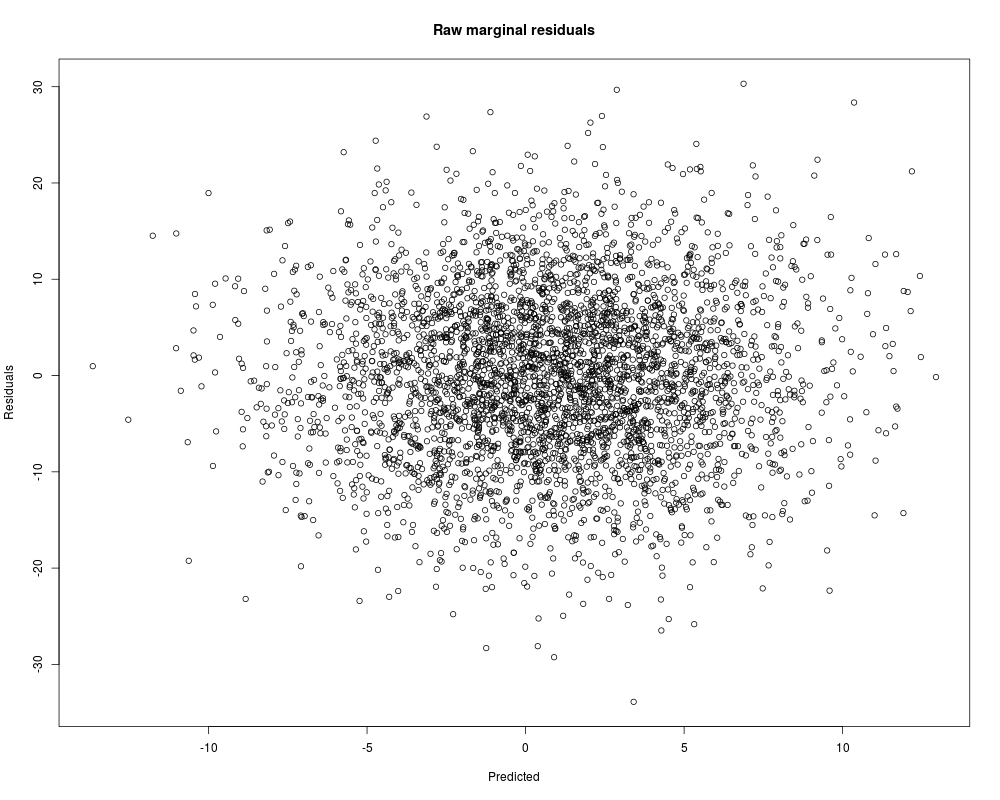
Distribution of marginal residuals
     Min.   1st Qu.    Median      Mean   3rd Qu.      Max. 
-33.89000  -5.78300  -0.05905   0.00000   5.85500  30.30000 

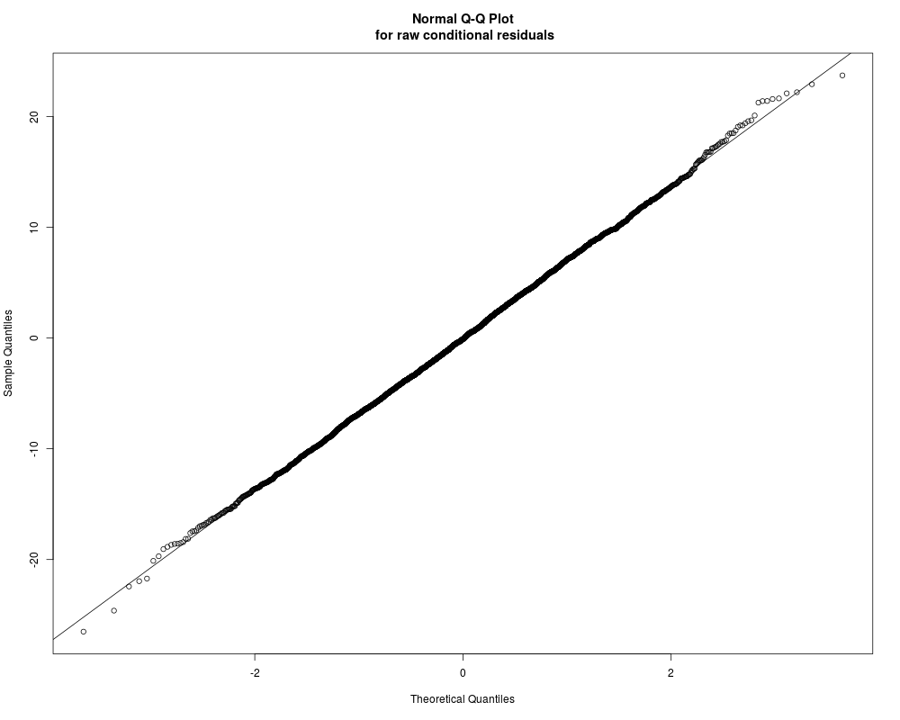
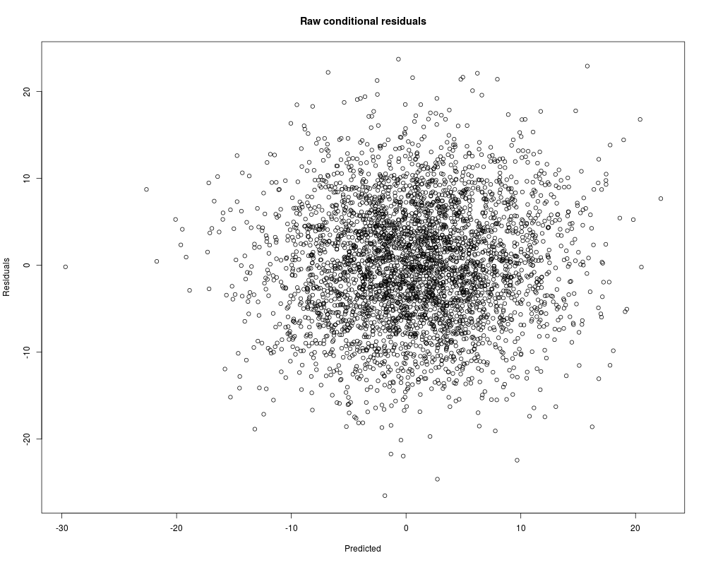
Distribution of raw conditional residuals
     Min.   1st Qu.    Median      Mean   3rd Qu.      Max. 
-26.51000  -4.67600  -0.09345   0.00000   4.64400  23.72000 

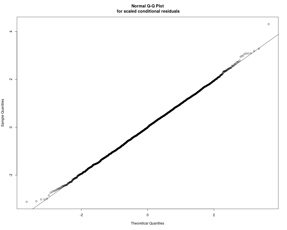
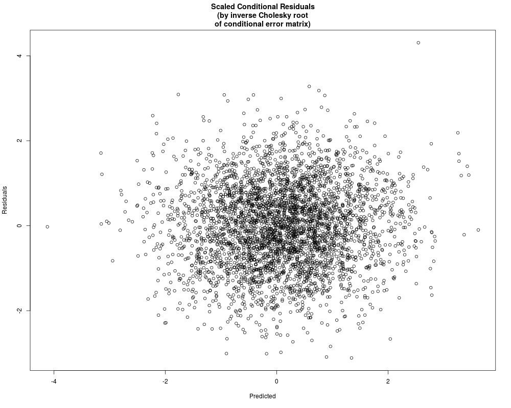
Distribution of scaled conditional residuals
     Min.   1st Qu.    Median      Mean   3rd Qu.      Max. 
-3.113000 -0.666000 -0.005821  0.000000  0.662500  4.308000 

> 
>  plot(result)
> ## End(No test)
> 
> 
> 
> 
> 
> dev.off()
null device 
          1 
>