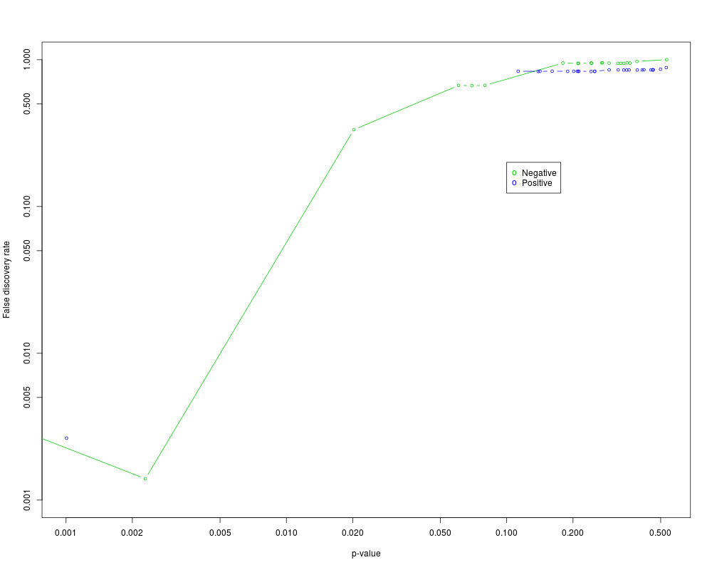
Plot the results from a Gene set analysis

Description

Plots the results from a call to GSA (Gene set analysis)

Usage

GSA.plot(GSA.obj, fac=1, FDRcut = 1)

Arguments

.

.

Details

This function makes a plot of the significant gene sets, based on a call to the GSA (Gene set analysis) function.

Author(s)

Robert Tibshirani

References

Efron, B. and Tibshirani, R. On testing the significance of sets of genes. Stanford tech report rep 2006. http://www-stat.stanford.edu/~tibs/ftp/GSA.pdf

Examples

######### two class unpaired comparison
# y must take values 1,2

set.seed(100)
x<-matrix(rnorm(1000*20),ncol=20)
dd<-sample(1:1000,size=100)

u<-matrix(2*rnorm(100),ncol=10,nrow=100)
x[dd,11:20]<-x[dd,11:20]+u
y<-c(rep(1,10),rep(2,10))


genenames=paste("g",1:1000,sep="")

#create some radnom gene sets
genesets=vector("list",50)
for(i in 1:50){
 genesets[[i]]=paste("g",sample(1:1000,size=30),sep="")
}
geneset.names=paste("set",as.character(1:50),sep="")

GSA.obj<-GSA(x,y, genenames=genenames, genesets=genesets,  resp.type="Two class unpaired", nperms=100)


GSA.listsets(GSA.obj, geneset.names=geneset.names,FDRcut=.5)

GSA.plot(GSA.obj)

Results

R version 3.3.1 (2016-06-21) -- "Bug in Your Hair"
Copyright (C) 2016 The R Foundation for Statistical Computing
Platform: x86_64-pc-linux-gnu (64-bit)

R is free software and comes with ABSOLUTELY NO WARRANTY.
You are welcome to redistribute it under certain conditions.
Type 'license()' or 'licence()' for distribution details.

R is a collaborative project with many contributors.
Type 'contributors()' for more information and
'citation()' on how to cite R or R packages in publications.

Type 'demo()' for some demos, 'help()' for on-line help, or
'help.start()' for an HTML browser interface to help.
Type 'q()' to quit R.

> library(GSA)
> png(filename="/home/ddbj/snapshot/RGM3/R_CC/result/GSA/GSA.plot.Rd_%03d_medium.png", width=480, height=480)
> ### Name: GSA.plot
> ### Title: Plot the results from a Gene set analysis
> ### Aliases: GSA.plot
> ### Keywords: univar survival ts nonparametric
> 
> ### ** Examples
> 
> 
> ######### two class unpaired comparison
> # y must take values 1,2
> 
> set.seed(100)
> x<-matrix(rnorm(1000*20),ncol=20)
> dd<-sample(1:1000,size=100)
> 
> u<-matrix(2*rnorm(100),ncol=10,nrow=100)
> x[dd,11:20]<-x[dd,11:20]+u
> y<-c(rep(1,10),rep(2,10))
> 
> 
> genenames=paste("g",1:1000,sep="")
> 
> #create some radnom gene sets
> genesets=vector("list",50)
> for(i in 1:50){
+  genesets[[i]]=paste("g",sample(1:1000,size=30),sep="")
+ }
> geneset.names=paste("set",as.character(1:50),sep="")
> 
> GSA.obj<-GSA(x,y, genenames=genenames, genesets=genesets,  resp.type="Two class unpaired", nperms=100)
perm= 10 / 100 
perm= 20 / 100 
perm= 30 / 100 
perm= 40 / 100 
perm= 50 / 100 
perm= 60 / 100 
perm= 70 / 100 
perm= 80 / 100 
perm= 90 / 100 
perm= 100 / 100 
> 
> 
> GSA.listsets(GSA.obj, geneset.names=geneset.names,FDRcut=.5)
$FDRcut
[1] 0.5

$negative
     Gene_set Gene_set_name Score     p-value FDR     
[1,] "11"     "set11"       "-0.3151" "0"     "0"     
[2,] "15"     "set15"       "-0.6354" "0"     "0"     
[3,] "50"     "set50"       "-0.3587" "0.02"  "0.3333"

$positive
     Gene_set Gene_set_name Score    p-value FDR
[1,] "6"      "set6"        "0.5037" "0"     "0"
[2,] "17"     "set17"       "0.7162" "0"     "0"
[3,] "31"     "set31"       "0.4192" "0"     "0"

$nsets.neg
[1] 3

$nsets.pos
[1] 3

> 
> GSA.plot(GSA.obj)
Warning messages:
1: In xy.coords(x, y, xlabel, ylabel, log) :
  1 x value <= 0 omitted from logarithmic plot
2: In xy.coords(x, y, xlabel, ylabel, log) :
  2 y values <= 0 omitted from logarithmic plot
> 
> 
> 
> 
> 
> 
> dev.off()
null device 
          1 
>