Estimate occurrence probabilities of a sampling plan (points)

Description

Estimates occurrence probabilities as an average between the kernel density estimation (spreading of points in geographical space) and MaxLike analysis (spreading of points in feature space). The output 'iprob' indicates whether the sampling plan has systematically missed some important locations / features, and can be used as an input for geostatistical modelling (e.g. as weights for regression modeling).

Usage

 
## S4 method for signature 'SpatialPoints,SpatialPixelsDataFrame'
spsample.prob(observations, covariates, 
  quant.nndist=.95, n.sigma, ...)

Arguments

Value

Returns a list of objects where 'iprob' ("SpatialPixelsDataFrame") is the map showing the estimated occurrence probabilities.

Note

Occurrence probabilities for geographical space are derived using kernel density estimator. The sampling intensities are converted to probabilities by deviding the sampling intensity by the maximum sampling intensity for the study area (Baddeley, 2008). The occurrence probabilities for feature space are determined using MaxLike algorithm (Royle et al., 2012). The lower the average occurrence probability for the whole study area, the lower the representation efficiency of a sampling plan.
MaxLike function might fail to produce predictions (e.g. if not at least one continuous covariate is provided and if the optim function is not able to find the global optima) in which case an error message is generated. Running Principal Component analysis i.e. standardizing the covariates prior to running spsample.prob is, thus, highly recommended.
This function can be time consuming for large grids.

Author(s)

Tomislav Hengl

References

• Baddeley, A. (2008) Analysing spatial point patterns in R. Technical report, CSIRO Australia. Version 4.

• Royle, J.A., Chandler, R.B., Yackulic, C. and J. D. Nichols. (2012) Likelihood analysis of species occurrence probability from presence-only data for modelling species distributions. Methods in Ecology and Evolution.

See Also

maxlike-package, spatstat-package

Examples

library(plotKML)
library(maxlike)
library(spatstat)
library(maptools)

data(eberg)
data(eberg_grid)
## existing sampling plan:
sel <- runif(nrow(eberg)) < .2
eberg.xy <- eberg[sel,c("X","Y")]
coordinates(eberg.xy) <- ~X+Y
proj4string(eberg.xy) <- CRS("+init=epsg:31467")
## covariates:
gridded(eberg_grid) <- ~x+y
proj4string(eberg_grid) <- CRS("+init=epsg:31467")
## convert to continuous independent covariates:
formulaString <- ~ PRMGEO6+DEMSRT6+TWISRT6+TIRAST6
eberg_spc <- spc(eberg_grid, formulaString)

## derive occurrence probability:
covs <- eberg_spc@predicted[1:8]
iprob <- spsample.prob(eberg.xy, covs)
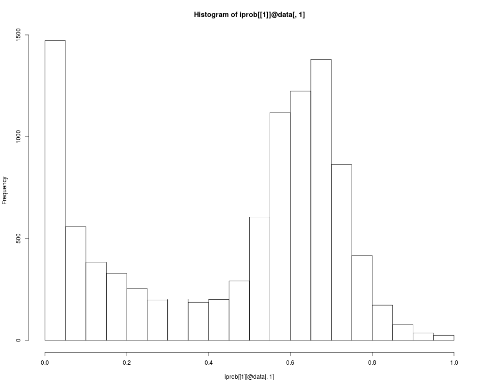
## Note: obvious omission areas:
hist(iprob[[1]]@data[,1])
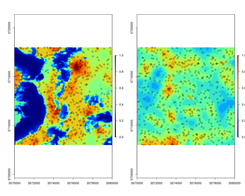
## compare with random sampling:
rnd <- spsample(eberg_grid, type="random",
     n=length(iprob[["observations"]]))
iprob2 <- spsample.prob(rnd, covs)
## compare the two:
par(mfrow=c(1,2))
plot(raster(iprob[[1]]), zlim=c(0,1), col=SAGA_pal[[1]])
points(iprob[["observations"]])
plot(raster(iprob2[[1]]), zlim=c(0,1), col=SAGA_pal[[1]])
points(iprob2[["observations"]])

## fit a weighted lm:
eberg.xy <- eberg[sel,c("SNDMHT_A","X","Y")]
coordinates(eberg.xy) <- ~X+Y
proj4string(eberg.xy) <- CRS("+init=epsg:31467")
eberg.xy$iprob <- over(eberg.xy, iprob[[1]])$iprob
eberg.xy@data <- cbind(eberg.xy@data, over(eberg.xy, covs))
fs <- as.formula(paste("SNDMHT_A ~ ", 
    paste(names(covs), collapse="+")))
## the lower the occurrence probability, the higher the weight:
w <- 1/eberg.xy$iprob
m <- lm(fs, eberg.xy, weights=w)
summary(m)
## compare to standard lm:
m0 <- lm(fs, eberg.xy)
summary(m)$adj.r.squared
summary(m0)$adj.r.squared

## all at once:
gm <- fit.gstatModel(eberg.xy, fs, covs, weights=w)
plot(gm)

Results

R version 3.3.1 (2016-06-21) -- "Bug in Your Hair"
Copyright (C) 2016 The R Foundation for Statistical Computing
Platform: x86_64-pc-linux-gnu (64-bit)

R is free software and comes with ABSOLUTELY NO WARRANTY.
You are welcome to redistribute it under certain conditions.
Type 'license()' or 'licence()' for distribution details.

R is a collaborative project with many contributors.
Type 'contributors()' for more information and
'citation()' on how to cite R or R packages in publications.

Type 'demo()' for some demos, 'help()' for on-line help, or
'help.start()' for an HTML browser interface to help.
Type 'q()' to quit R.

> library(GSIF)
GSIF version 0.5-2 (2016-06-25)
URL: http://gsif.r-forge.r-project.org/
> png(filename="/home/ddbj/snapshot/RGM3/R_CC/result/GSIF/spsample.prob.Rd_%03d_medium.png", width=480, height=480)
> ### Name: spsample.prob
> ### Title: Estimate occurrence probabilities of a sampling plan (points)
> ### Aliases: spsample.prob
> ###   spsample.prob,SpatialPoints,SpatialPixelsDataFrame-method
> 
> ### ** Examples
> 
> library(plotKML)
plotKML version 0.5-6 (2016-05-02)
URL: http://plotkml.r-forge.r-project.org/
> library(maxlike)
Loading required package: raster
Loading required package: sp
> library(spatstat)
Loading required package: nlme

Attaching package: 'nlme'

The following object is masked from 'package:raster':

    getData

Loading required package: rpart

spatstat 1.45-2       (nickname: 'Caretaker Mode') 
For an introduction to spatstat, type 'beginner' 


Attaching package: 'spatstat'

The following objects are masked from 'package:raster':

    area, rotate, shift

> library(maptools)
Checking rgeos availability: TRUE
> 
> data(eberg)
> data(eberg_grid)
> ## existing sampling plan:
> sel <- runif(nrow(eberg)) < .2
> eberg.xy <- eberg[sel,c("X","Y")]
> coordinates(eberg.xy) <- ~X+Y
> proj4string(eberg.xy) <- CRS("+init=epsg:31467")
> ## covariates:
> gridded(eberg_grid) <- ~x+y
> proj4string(eberg_grid) <- CRS("+init=epsg:31467")
> ## convert to continuous independent covariates:
> formulaString <- ~ PRMGEO6+DEMSRT6+TWISRT6+TIRAST6
> eberg_spc <- spc(eberg_grid, formulaString)
Converting PRMGEO6 to indicators...
Converting covariates to principal components...
Warning message:
In prcomp.default(formula = formulaString, x) :
 extra argument 'formula' will be disregarded 
> 
> ## derive occurrence probability:
> covs <- eberg_spc@predicted[1:8]
> iprob <- spsample.prob(eberg.xy, covs)
Deriving kernel density map using sigma 354 ...
Deriving inclusion probabilities using MaxLike analysis...
> ## Note: obvious omission areas:
> hist(iprob[[1]]@data[,1])
> ## compare with random sampling:
> rnd <- spsample(eberg_grid, type="random",
+      n=length(iprob[["observations"]]))
> iprob2 <- spsample.prob(rnd, covs)
Deriving kernel density map using sigma 438 ...
Deriving inclusion probabilities using MaxLike analysis...
> ## compare the two:
> par(mfrow=c(1,2))
> plot(raster(iprob[[1]]), zlim=c(0,1), col=SAGA_pal[[1]])
> points(iprob[["observations"]])
> plot(raster(iprob2[[1]]), zlim=c(0,1), col=SAGA_pal[[1]])
> points(iprob2[["observations"]])
> 
> ## fit a weighted lm:
> eberg.xy <- eberg[sel,c("SNDMHT_A","X","Y")]
> coordinates(eberg.xy) <- ~X+Y
> proj4string(eberg.xy) <- CRS("+init=epsg:31467")
> eberg.xy$iprob <- over(eberg.xy, iprob[[1]])$iprob
> eberg.xy@data <- cbind(eberg.xy@data, over(eberg.xy, covs))
> fs <- as.formula(paste("SNDMHT_A ~ ", 
+     paste(names(covs), collapse="+")))
> ## the lower the occurrence probability, the higher the weight:
> w <- 1/eberg.xy$iprob
> m <- lm(fs, eberg.xy, weights=w)
> summary(m)

Call:
lm(formula = fs, data = eberg.xy, weights = w)

Weighted Residuals:
    Min      1Q  Median      3Q     Max 
-63.424 -11.422  -0.756   8.252  78.642 

Coefficients:
            Estimate Std. Error t value Pr(>|t|)    
(Intercept)  28.0546     0.7827  35.845  < 2e-16 ***
PC1           1.3767     0.6003   2.293   0.0222 *  
PC2          -4.3319     0.5335  -8.120 2.93e-15 ***
PC3           4.7445     0.6702   7.079 4.33e-12 ***
PC4         -10.0059     0.5256 -19.038  < 2e-16 ***
PC5          -2.9031     0.5073  -5.723 1.70e-08 ***
PC6          -0.3242     0.6201  -0.523   0.6013    
PC7          -1.0757     0.4678  -2.299   0.0218 *  
PC8          -3.7207     0.6913  -5.382 1.08e-07 ***
---
Signif. codes:  0 '***' 0.001 '**' 0.01 '*' 0.05 '.' 0.1 ' ' 1

Residual standard error: 18.55 on 565 degrees of freedom
  (183 observations deleted due to missingness)
Multiple R-squared:  0.491,	Adjusted R-squared:  0.4837 
F-statistic: 68.11 on 8 and 565 DF,  p-value: < 2.2e-16

> ## compare to standard lm:
> m0 <- lm(fs, eberg.xy)
> summary(m)$adj.r.squared
[1] 0.483744
> summary(m0)$adj.r.squared
[1] 0.470544
> 
> ## all at once:
> gm <- fit.gstatModel(eberg.xy, fs, covs, weights=w)
Fitting a linear model...
Warning: Shapiro-Wilk normality test and Anderson-Darling normality test report probability of < .05 indicating lack of normal distribution for residuals
Fitting a 2D variogram...
Saving an object of class 'gstatModel'...
Warning message:
In gstat::fit.variogram(svgm, model = ivgm, ...) :
  No convergence after 200 iterations: try different initial values?
> plot(gm)
Error in dev.new(width = 9, height = 5) : 
  no suitable unused file name for pdf()
Calls: plot -> plot -> dev.new
Execution halted