R Graphical Manual

Browse All

Last data update: 2014.03.03

R: Plot of a Gamma Shape Mixture Model

plot-methods

R Documentation

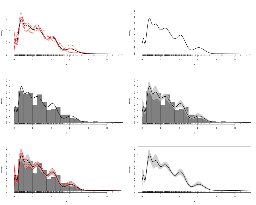
Plot of a Gamma Shape Mixture Model

Description

plot method for class "gsm". This function plots the output of a Gamma Shape Mixture estimation procedure.

Usage

## S4 method for signature 'gsm,missing'
plot(x, ndens = 5, xlab = "x", ylab = "density", nbin = 10,
		histogram = FALSE, bands = FALSE, confid = .95, start = 1, ...)

Arguments

`x`	object of class "gsm"; a list returned by the `estim.gsm` or `estim.gsm_theta` functions.
`ndens`	number of simulated density curves to plot.
`xlab`	a title for the x axis.
`ylab`	a title for the y axis.
`nbin`	number of bins for the histogram.
`histogram`	logical; if TRUE the histogram is plotted on the figure.
`bands`	logical; if TRUE the 95% credibility bands are overimposed on the density graph.
`confid`	confidence level for the pointwise credibility bands around the density estimate.
`start`	MCMC run to start from.
`...`	further arguments passed to or from other methods.

Details

To produce a standard histogram with the estimated density curve superimposed on it, simply set ndens to 0 and histogram to TRUE.

Value

List with the following components:

`xval`	horizontal coordinates.
`yval`	vertical coordinates (pointwise density posterior means).

Author(s)

Sergio Venturini sergio.venturini@unibocconi.it

References

Venturini, S., Dominici, F. and Parmigiani, G. (2008), "Gamma shape mixtures for heavy-tailed distributions". Annals of Applied Statistics, Volume 2, Number 2, 756–776. http://projecteuclid.org/euclid.aoas/1215118537

Examples

set.seed(2040)
y <- rgsm(500, c(.1, .3, .4, .2), 1)
burnin <- 5
mcmcsim <- 10
J <- 250
gsm.out <- estim.gsm(y, J, 300, burnin + mcmcsim, 6500, 340, 1/J)
par(mfrow = c(3, 2))
plot(gsm.out)
plot(gsm.out, ndens = 0, nbin = 20, start = (burnin + 1))
plot(gsm.out, ndens = 0, nbin = 20, histogram = TRUE, start = (burnin + 1))
plot(gsm.out, ndens = 0, nbin = 20, histogram = TRUE, bands = TRUE, start = (burnin + 1))
plot(gsm.out, ndens = 5, nbin = 20, histogram = TRUE, bands = TRUE, start = (burnin + 1))
plot(gsm.out, ndens = 0, nbin = 20, bands = TRUE, start = (burnin + 1))

Results


R version 3.3.1 (2016-06-21) -- "Bug in Your Hair"
Copyright (C) 2016 The R Foundation for Statistical Computing
Platform: x86_64-pc-linux-gnu (64-bit)

R is free software and comes with ABSOLUTELY NO WARRANTY.
You are welcome to redistribute it under certain conditions.
Type 'license()' or 'licence()' for distribution details.

R is a collaborative project with many contributors.
Type 'contributors()' for more information and
'citation()' on how to cite R or R packages in publications.

Type 'demo()' for some demos, 'help()' for on-line help, or
'help.start()' for an HTML browser interface to help.
Type 'q()' to quit R.

> library(GSM)
Loading required package: gtools
Package GSM (1.3.2) loaded.
To cite, see citation("GSM")

> png(filename="/home/ddbj/snapshot/RGM3/R_CC/result/GSM/plot-methods.Rd_%03d_medium.png", width=480, height=480)
> ### Name: plot-methods
> ### Title: Plot of a Gamma Shape Mixture Model
> ### Aliases: plot-methods plot,ANY,ANY-method plot,gsm,missing-method
> ### Keywords: methods
> 
> ### ** Examples
> 
> set.seed(2040)
> y <- rgsm(500, c(.1, .3, .4, .2), 1)
> burnin <- 5
> mcmcsim <- 10
> J <- 250
> gsm.out <- estim.gsm(y, J, 300, burnin + mcmcsim, 6500, 340, 1/J)
> par(mfrow = c(3, 2))
> plot(gsm.out)
> plot(gsm.out, ndens = 0, nbin = 20, start = (burnin + 1))
> plot(gsm.out, ndens = 0, nbin = 20, histogram = TRUE, start = (burnin + 1))
> plot(gsm.out, ndens = 0, nbin = 20, histogram = TRUE, bands = TRUE, start = (burnin + 1))
> plot(gsm.out, ndens = 5, nbin = 20, histogram = TRUE, bands = TRUE, start = (burnin + 1))
> plot(gsm.out, ndens = 0, nbin = 20, bands = TRUE, start = (burnin + 1))
> 
> 
> 
> 
> 
> dev.off()
null device 
          1 
>