R Graphical Manual

Browse All

Last data update: 2014.03.03

R: EM-PAVA function

EM_PAVA_Func

R Documentation

EM-PAVA function

Description

This function is used to estimate the genotype-specific distribution of time-to-event outcomes using EM-PAVA algorithm (Qin et al. 2014).

Usage

EM_PAVA_Func (q, x, delta, timeval, p, ep = 1e-05, maxiter = 400)

Arguments

`q`	matrix of 2 columns, where the first and second columns are the probabilities of belonging to the carrier `p0G` and non-carrier groups `1 - p0G`, respectively.
`x`	observed event time or censoring time.
`delta`	indicator of event.
`timeval`	grid points at which the distribution function values are estimated.
`p`	number of groups.
`ep`	convergence criterion. Here, `ep = 1e-5` is used as the default value.
`maxiter`	maximum number of EM iterations.

Details

Technical details can be found in Qin et al. (2014).

Value

Returns a list of prediction values for classes

`Fest`	estimated values at the points of `timeval`.
`Fest.all`	estimated values of cumulative distribution function on both carrier and non-carrier groups.

References

Qin, J., Garcia, T., Ma, Y., Tang, M., Marder, K. & Wang, Y. (2014). Combining isotonic regression and EM algorithm to predict genetic risk under monotonicity constraint. The Annals of Applied Statistics 8(2), 1182-1208.

Examples


data("Simulated_data");

OY = Simulated_data[,2];
ind = order(OY);
ODelta = Simulated_data[,3];
Op0G = Simulated_data[,4];

Y = OY[ind];
Delta = ODelta[ind];
p0G = Op0G[ind];

Grid = seq(0.01, 3.65, 0.01);
fix_t1 = c(0.288, 0.693, 1.390);
fix_t2 = c(0.779, 1.860, 3.650);

EMpava_result = EM_PAVA_Func ( q = rbind(p0G,1-p0G), x = Y, delta = Delta, 
                               timeval = Grid, p = 2, ep = 1e-4 );

all = sort(c(Grid, Y));

F_carr_func = function(x){  EMpava_result$Fest.all[1, which.max(all[all <= x]) ]  };
F_non_func  = function(x){  EMpava_result$Fest.all[2, which.max(all[all <= x]) ]  };

PAVA_F1.hat_fix_t = apply( matrix(fix_t1, ncol=1), 1, F_carr_func );
PAVA_F2.hat_fix_t = apply( matrix(fix_t2, ncol=1), 1, F_non_func );

PAVA_F.hat_fix_t = data.frame( fix_t1 = fix_t1, PAVA_F1.hat = PAVA_F1.hat_fix_t,
                               fix_t2 = fix_t2, PAVA_F2.hat = PAVA_F2.hat_fix_t  );

print(PAVA_F.hat_fix_t);

# plot estimated curves

F_carr = apply( matrix(Grid, ncol=1), 1, F_carr_func );
F_non = apply( matrix(Grid, ncol=1), 1, F_non_func );

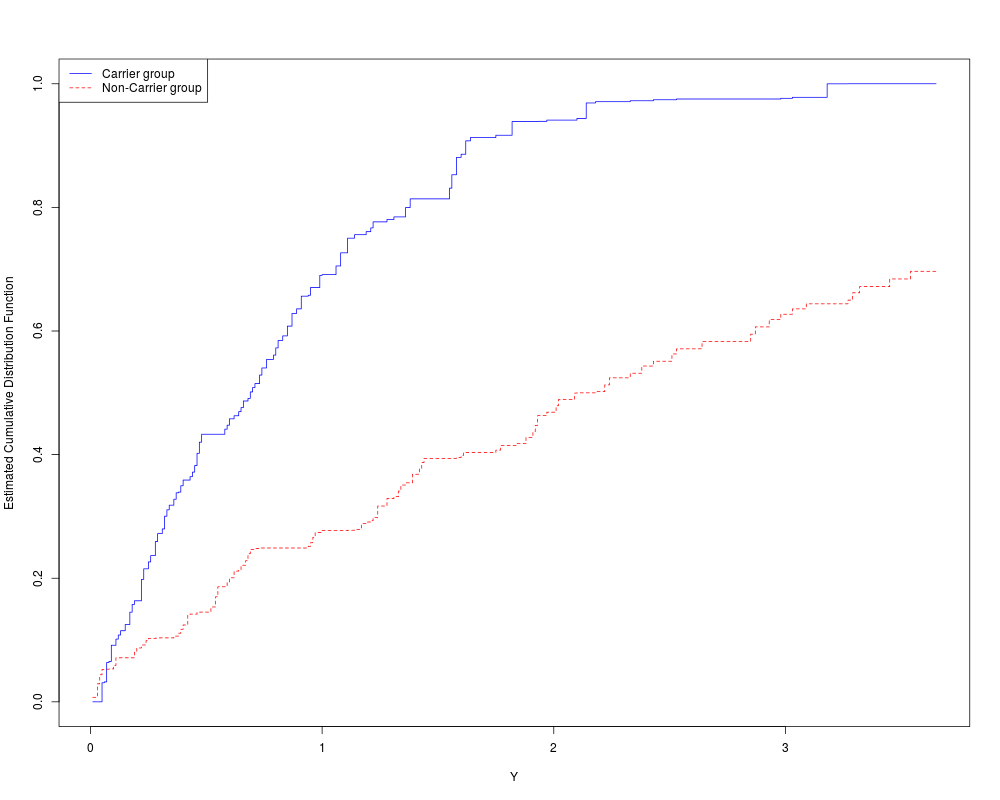
plot( Grid, F_carr, type = 's', lty = 1, 
      xlab = "Y", ylab = "Estimated Cumulative Distribution Function",
      ylim = c(0,1), col = 'blue' );
lines(Grid, F_non, type='s', lty=2, col='red');
legend("topleft", legend=c("Carrier group", "Non-Carrier group"),
       lty=c(1,2), col=c("blue", "red") );

Results


R version 3.3.1 (2016-06-21) -- "Bug in Your Hair"
Copyright (C) 2016 The R Foundation for Statistical Computing
Platform: x86_64-pc-linux-gnu (64-bit)

R is free software and comes with ABSOLUTELY NO WARRANTY.
You are welcome to redistribute it under certain conditions.
Type 'license()' or 'licence()' for distribution details.

R is a collaborative project with many contributors.
Type 'contributors()' for more information and
'citation()' on how to cite R or R packages in publications.

Type 'demo()' for some demos, 'help()' for on-line help, or
'help.start()' for an HTML browser interface to help.
Type 'q()' to quit R.

> library(GSSE)
> png(filename="/home/ddbj/snapshot/RGM3/R_CC/result/GSSE/EM_PAVA_Func.Rd_%03d_medium.png", width=480, height=480)
> ### Name: EM_PAVA_Func
> ### Title: EM-PAVA function
> ### Aliases: EM_PAVA_Func
> 
> ### ** Examples
> 
> 
> data("Simulated_data");
> 
> OY = Simulated_data[,2];
> ind = order(OY);
> ODelta = Simulated_data[,3];
> Op0G = Simulated_data[,4];
> 
> Y = OY[ind];
> Delta = ODelta[ind];
> p0G = Op0G[ind];
> 
> Grid = seq(0.01, 3.65, 0.01);
> fix_t1 = c(0.288, 0.693, 1.390);
> fix_t2 = c(0.779, 1.860, 3.650);
> 
> EMpava_result = EM_PAVA_Func ( q = rbind(p0G,1-p0G), x = Y, delta = Delta, 
+                                timeval = Grid, p = 2, ep = 1e-4 );
> 
> all = sort(c(Grid, Y));
> 
> F_carr_func = function(x){  EMpava_result$Fest.all[1, which.max(all[all <= x]) ]  };
> F_non_func  = function(x){  EMpava_result$Fest.all[2, which.max(all[all <= x]) ]  };
> 
> PAVA_F1.hat_fix_t = apply( matrix(fix_t1, ncol=1), 1, F_carr_func );
> PAVA_F2.hat_fix_t = apply( matrix(fix_t2, ncol=1), 1, F_non_func );
> 
> PAVA_F.hat_fix_t = data.frame( fix_t1 = fix_t1, PAVA_F1.hat = PAVA_F1.hat_fix_t,
+                                fix_t2 = fix_t2, PAVA_F2.hat = PAVA_F2.hat_fix_t  );
> 
> print(PAVA_F.hat_fix_t);
  fix_t1 PAVA_F1.hat fix_t2 PAVA_F2.hat
1  0.288   0.2696055  0.779   0.2488954
2  0.693   0.5084504  1.860   0.4177679
3  1.390   0.8137684  3.650   0.6965440
> 
> # plot estimated curves
> 
> F_carr = apply( matrix(Grid, ncol=1), 1, F_carr_func );
> F_non = apply( matrix(Grid, ncol=1), 1, F_non_func );
> 
> plot( Grid, F_carr, type = 's', lty = 1, 
+       xlab = "Y", ylab = "Estimated Cumulative Distribution Function",
+       ylim = c(0,1), col = 'blue' );
> lines(Grid, F_non, type='s', lty=2, col='red');
> legend("topleft", legend=c("Carrier group", "Non-Carrier group"),
+        lty=c(1,2), col=c("blue", "red") );
> 
> 
> 
> 
> 
> 
> dev.off()
null device 
          1 
>