Generalized UniFrac distances for comparing microbial communities.

Description

A generalized version of commonly used UniFrac distances. It is defined as:

d^{(α)} = [∑_{i=1}^m b_i (p^A_{i} + p^B_{i})^α |p^A_{i} - p^B_{i}|/(p^A_{i} + p^B_{i})]/ [ ∑_{i=1}^m b_i (p^A_{i} + p^B_{i})^α],

where m is the number of branches, b_i is the length of ith branch, p^A_{i}, p^B_{i} are the branch proportion for community A and B.

Generalized UniFrac distance contains an extra parameter α controlling the weight on abundant lineages so the distance is not dominated by highly abundant lineages. α=0.5 has overall the best power.

The unweighted and weighted UniFrac, and variance adjusted weighted UniFrac distances are also implemented.

Usage

GUniFrac(otu.tab, tree, alpha = c(0, 0.5, 1))

Arguments

Value

Return a LIST containing

Note

The function only accepts rooted tree. To root a tree, you may consider using the R code from https://stat.ethz.ch/pipermail/r-sig-phylo/2010-September/000750.html

Author(s)

Jun Chen <chenjun@mail.med.upenn.edu>

References

Jun Chen and Hongzhe Li(2012). Associating microbiome composition with environmental covariates using generalized UniFrac distances. (Submitted)

See Also

Rarefy, PermanovaG

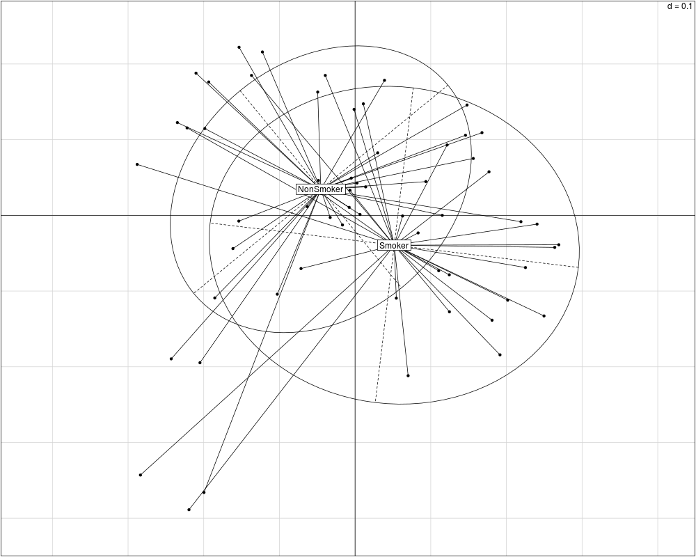
Examples

require(ade4)

data(throat.otu.tab)
data(throat.tree)
data(throat.meta)

groups <- throat.meta$SmokingStatus

# Rarefaction
otu.tab.rff <- Rarefy(throat.otu.tab)$otu.tab.rff

# Calculate the UniFracs
unifracs <- GUniFrac(otu.tab.rff, throat.tree, alpha=c(0, 0.5, 1))$unifracs

dw <- unifracs[, , "d_1"]		# Weighted UniFrac
du <- unifracs[, , "d_UW"]		# Unweighted UniFrac	
dv <- unifracs[, , "d_VAW"]		# Variance adjusted weighted UniFrac
d0 <- unifracs[, , "d_0"]     		# GUniFrac with alpha 0  
d5 <- unifracs[, , "d_0.5"]   		# GUniFrac with alpha 0.5 

# Permanova - Distance based multivariate analysis of variance
adonis(as.dist(d5) ~ groups)

# PCoA plot
s.class(cmdscale(d5, k=2), fac = groups) 

Results

R version 3.3.1 (2016-06-21) -- "Bug in Your Hair"
Copyright (C) 2016 The R Foundation for Statistical Computing
Platform: x86_64-pc-linux-gnu (64-bit)

R is free software and comes with ABSOLUTELY NO WARRANTY.
You are welcome to redistribute it under certain conditions.
Type 'license()' or 'licence()' for distribution details.

R is a collaborative project with many contributors.
Type 'contributors()' for more information and
'citation()' on how to cite R or R packages in publications.

Type 'demo()' for some demos, 'help()' for on-line help, or
'help.start()' for an HTML browser interface to help.
Type 'q()' to quit R.

> library(GUniFrac)
Loading required package: vegan
Loading required package: permute
Loading required package: lattice
This is vegan 2.4-0
Loading required package: ape
> png(filename="/home/ddbj/snapshot/RGM3/R_CC/result/GUniFrac/GUniFrac.Rd_%03d_medium.png", width=480, height=480)
> ### Name: GUniFrac
> ### Title: Generalized UniFrac distances for comparing microbial
> ###   communities.
> ### Aliases: GUniFrac
> ### Keywords: distance UniFrac ecology
> 
> ### ** Examples
> 
> require(ade4)
Loading required package: ade4

Attaching package: 'ade4'

The following object is masked from 'package:vegan':

    cca

> 
> data(throat.otu.tab)
> data(throat.tree)
> data(throat.meta)
> 
> groups <- throat.meta$SmokingStatus
> 
> # Rarefaction
> otu.tab.rff <- Rarefy(throat.otu.tab)$otu.tab.rff
> 
> # Calculate the UniFracs
> unifracs <- GUniFrac(otu.tab.rff, throat.tree, alpha=c(0, 0.5, 1))$unifracs
> 
> dw <- unifracs[, , "d_1"]		# Weighted UniFrac
> du <- unifracs[, , "d_UW"]		# Unweighted UniFrac	
> dv <- unifracs[, , "d_VAW"]		# Variance adjusted weighted UniFrac
> d0 <- unifracs[, , "d_0"]     		# GUniFrac with alpha 0  
> d5 <- unifracs[, , "d_0.5"]   		# GUniFrac with alpha 0.5 
> 
> # Permanova - Distance based multivariate analysis of variance
> adonis(as.dist(d5) ~ groups)

Call:
adonis(formula = as.dist(d5) ~ groups) 

Permutation: free
Number of permutations: 999

Terms added sequentially (first to last)

          Df SumsOfSqs MeanSqs F.Model      R2 Pr(>F)   
groups     1    0.3500 0.35004   2.501 0.04134  0.002 **
Residuals 58    8.1179 0.13996         0.95866          
Total     59    8.4680                 1.00000          
---
Signif. codes:  0 '***' 0.001 '**' 0.01 '*' 0.05 '.' 0.1 ' ' 1
> 
> # PCoA plot
> s.class(cmdscale(d5, k=2), fac = groups) 
> 
> 
> 
> 
> 
> 
> dev.off()
null device 
          1 
>