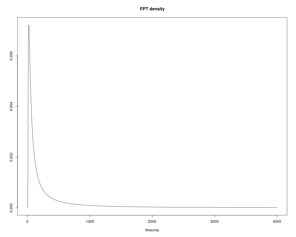
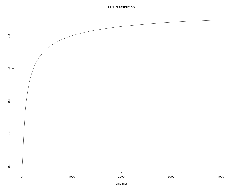
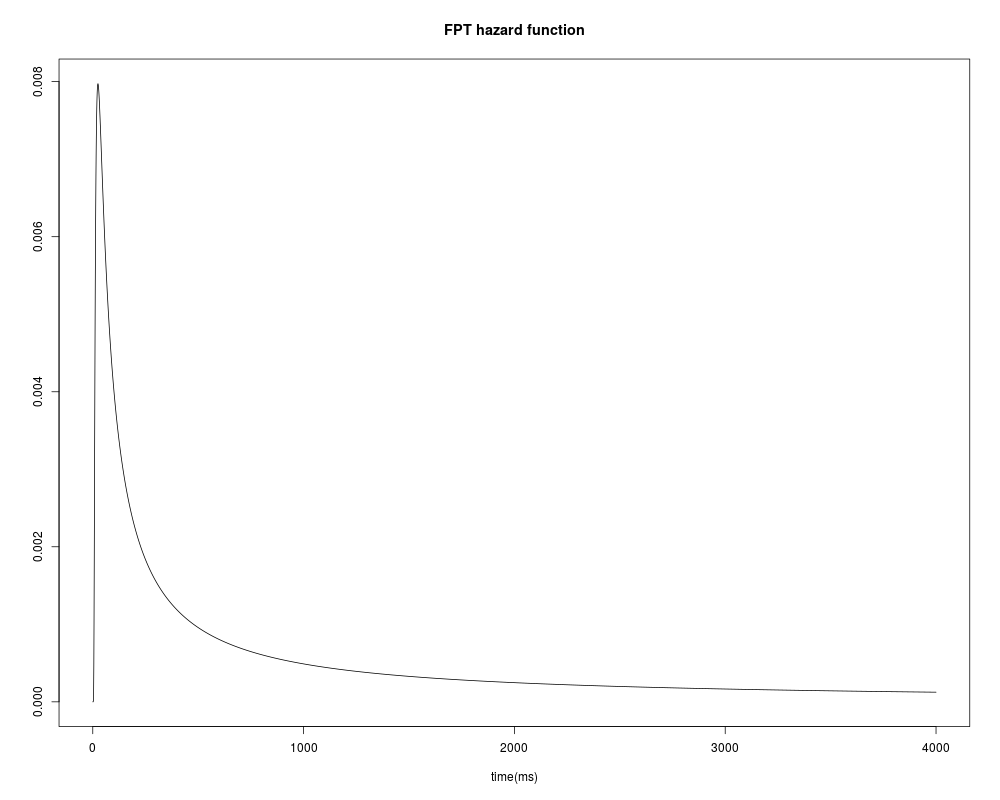
Evaluation of the FPT density and distribution functions

Description

The FPT density g0 and distribution function gg0 are evaluated up to a fixed time T on N1max gridpoints by numerical integration of the Volterra integral equation given in Buonocore 1987. Note that this time may not correspond to the final time Tfin when full reconstruction of the FPT density by quadrature is not required (quadflag set to 0 in the input parameters list).

Usage

FPTdensity_byint(obj,n1max)

Arguments

Value

Values are returned as an object of class “FPTdensity” yielding the timegrid and the corresponding values of the FPT density and FPT distribution.

Author(s)

A. Buonocore, M.F. Carfora

References

Buonocore, A., Nobile, A.G., and Ricciardi, L.M., A new integral equation for the evaluation of first-passage-time probability densities. Adv Appl Prob 19 (1987), 784–800.

Examples

##---- Should be DIRECTLY executable !! ----
##-- ==>  Define data, use random,
##--	or do  help(data=index)  for the standard data sets.

## Continuing the Wiener() example:


Nmax <- which.min(abs(mp[2:(N+1)]-mp[1:N]))
N1 <- N
if (quadflag == 0)   N1 <- max(c(Nmax,N/4))
N1p1 <- N1+1
answer <- FPTdensity_byint(param,N1)
plot(answer)

Results

R version 3.3.1 (2016-06-21) -- "Bug in Your Hair"
Copyright (C) 2016 The R Foundation for Statistical Computing
Platform: x86_64-pc-linux-gnu (64-bit)

R is free software and comes with ABSOLUTELY NO WARRANTY.
You are welcome to redistribute it under certain conditions.
Type 'license()' or 'licence()' for distribution details.

R is a collaborative project with many contributors.
Type 'contributors()' for more information and
'citation()' on how to cite R or R packages in publications.

Type 'demo()' for some demos, 'help()' for on-line help, or
'help.start()' for an HTML browser interface to help.
Type 'q()' to quit R.

> library(GaDiFPT)
> png(filename="/home/ddbj/snapshot/RGM3/R_CC/result/GaDiFPT/FPTdensity_byint.Rd_%03d_medium.png", width=480, height=480)
> ### Name: FPTdensity_byint
> ### Title: Evaluation of the FPT density and distribution functions
> ### Aliases: FPTdensity_byint
> 
> ### ** Examples
> 
> ##---- Should be DIRECTLY executable !! ----
> ##-- ==>  Define data, use random,
> ##--	or do  help(data=index)  for the standard data sets.
> 
> ## Continuing the Wiener() example:
> ## Don't show: 
> library(GaDiFPT)
> Wiener <- diffusion(c("mu","sigma2"))
> 
> # user-provided parameters and functions
> mu <- 0.0
> sigma2 <- 1.0
> Scost <- 8
> Sslope <- 0
> Stype <- "constant"
> 
> t0 <- 0.0
> x0 <- 0.0
> Tfin <- 4000    
> deltat <- 1.0
> N <- floor((Tfin - t0)/deltat)  
> M <- 1000
> quadflag <- 1
> RStudioflag <- TRUE
> 
> param <- inputlist(mu,sigma2,Stype,t0,x0,Tfin,deltat,M,quadflag,RStudioflag)
> 
> aaa <- function(t) {
+   aaa <- 0.0 + 0.0*t
+ }
> 
> bbb <- function(t) {
+   bbb <- mu + 0.0*t
+ }
> 
> SSS <- function(t) {
+   SSS <- Scost + Sslope*t
+ }
> 
> SSSp <- function(t) {
+   SSSp <- Sslope
+ }
> 
> ####       INITIALIZATION OF VECTORS
> 
> tempi <- numeric(N+1)
> mp <- numeric(N+1)
> up <- numeric(N+1)
> vp <- numeric(N+1)
> 
> # dummy vector
> app <- numeric(N)
> 
> ####    EVALUATION OF MEAN AND COVARIANCE OF THE PROCESS
> 
> tempi <- seq(t0, by=deltat, length=N+1)
> 
> dum <- vectorsetup(param)
> mp <- dum[,1]
> up <- dum[,2]
> vp <- dum[,3]
> ## End(Don't show)
> 
> Nmax <- which.min(abs(mp[2:(N+1)]-mp[1:N]))
> N1 <- N
> if (quadflag == 0)   N1 <- max(c(Nmax,N/4))
> N1p1 <- N1+1
> answer <- FPTdensity_byint(param,N1)
> plot(answer)
> 
> 
> 
> 
> 
> dev.off()
null device 
          1 
>