Supported by Dr. Osamu Ogasawara and  . . |
|
Last data update: 2014.03.03 |
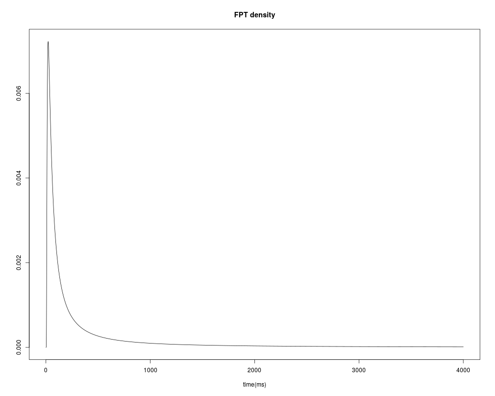
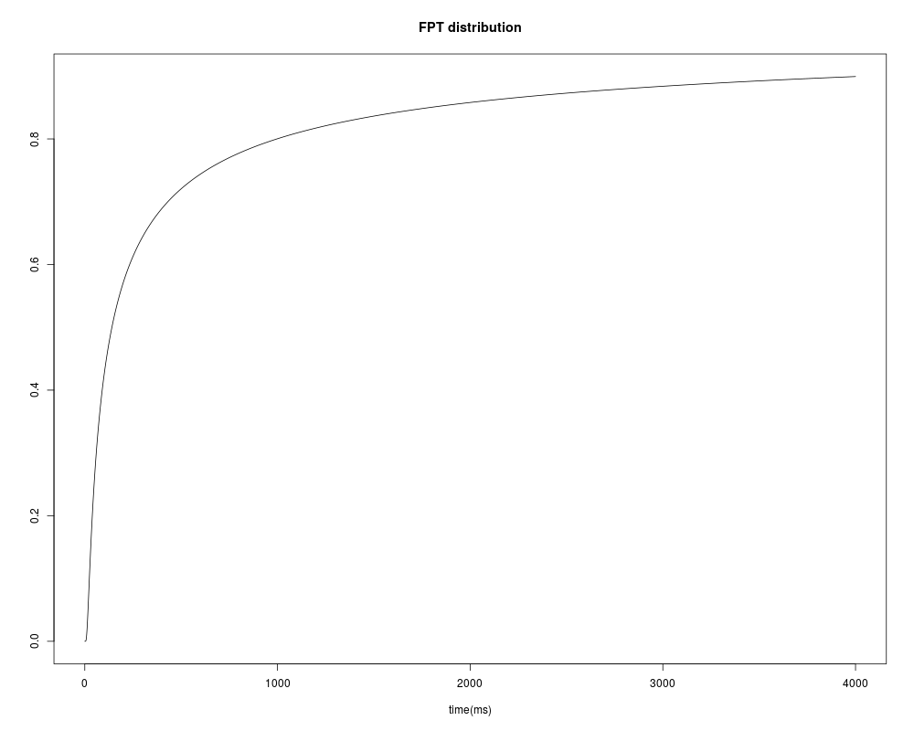
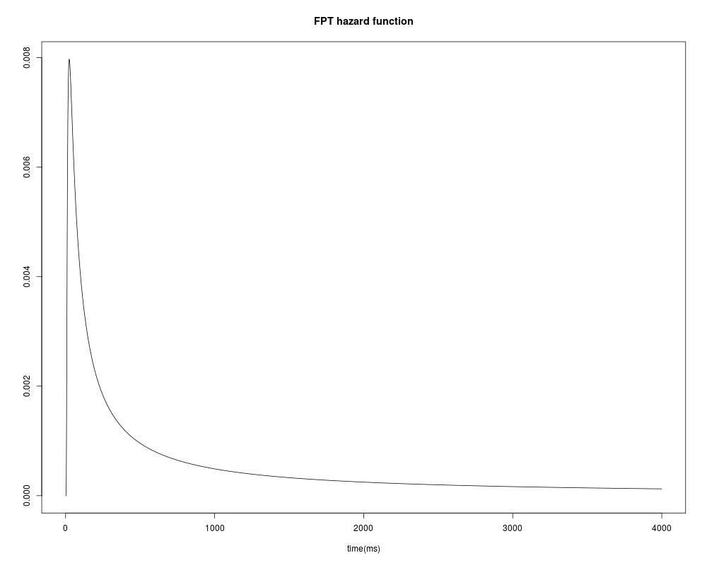
Simulation of FPT by the Hazard Rate MethodDescription
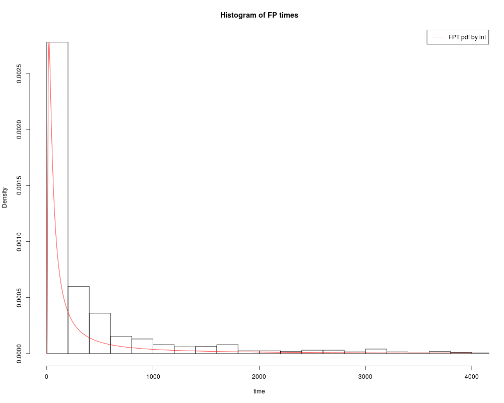
UsageFPTsimul(obj,M) histplot(obj1,obj) Arguments
Value
Author(s)A. Buonocore, M.F. Carfora ReferencesA. Buonocore, L. Caputo, E. Pirozzi, M.F. Carfora, A Simple Algorithm to Generate Firing Times for Leaky Integrate-and-Fire Neuronal Model, Math Biosci Eng,11, 1-10 (2014). Examples##---- Should be DIRECTLY executable !! ---- ##-- ==> Define data, use random, ##-- or do help(data=index) for the standard data sets. ## Continuing the Wiener() example: spikes <- FPTsimul(answer,M) histplot(spikes,answer) Results
R version 3.3.1 (2016-06-21) -- "Bug in Your Hair"
Copyright (C) 2016 The R Foundation for Statistical Computing
Platform: x86_64-pc-linux-gnu (64-bit)

R is free software and comes with ABSOLUTELY NO WARRANTY.
You are welcome to redistribute it under certain conditions.
Type 'license()' or 'licence()' for distribution details.

R is a collaborative project with many contributors.
Type 'contributors()' for more information and
'citation()' on how to cite R or R packages in publications.

Type 'demo()' for some demos, 'help()' for on-line help, or
'help.start()' for an HTML browser interface to help.
Type 'q()' to quit R.

> library(GaDiFPT)
> png(filename="/home/ddbj/snapshot/RGM3/R_CC/result/GaDiFPT/FPTsimul.Rd_%03d_medium.png", width=480, height=480)
> ### Name: FPTsimul
> ### Title: Simulation of FPT by the Hazard Rate Method
> ### Aliases: FPTsimul histplot
>
> ### ** Examples
>
> ##---- Should be DIRECTLY executable !! ----
> ##-- ==>  Define data, use random,
> ##--	or do  help(data=index)  for the standard data sets.
>
> ## Continuing the Wiener() example:
> ## Don't show:
> library(GaDiFPT)
> Wiener <- diffusion(c("mu","sigma2"))
>
> # user-provided parameters and functions
> mu <- 0.0
> sigma2 <- 1.0
> Scost <- 8
> Sslope <- 0
> Stype <- "constant"
>
> t0 <- 0.0
> x0 <- 0.0
> Tfin <- 4000
> deltat <- 1.0
> N <- floor((Tfin - t0)/deltat)
> M <- 1000
> quadflag <- 1
> RStudioflag <- TRUE
>
> param <- inputlist(mu,sigma2,Stype,t0,x0,Tfin,deltat,M,quadflag,RStudioflag)
>
> aaa <- function(t) {
+   aaa <- 0.0 + 0.0*t
+ }
>
> bbb <- function(t) {
+   bbb <- mu + 0.0*t
+ }
>
> SSS <- function(t) {
+   SSS <- Scost + Sslope*t
+ }
>
> SSSp <- function(t) {
+   SSSp <- Sslope
+ }
>
> ####       INITIALIZATION OF VECTORS
>
> tempi <- numeric(N+1)
> mp <- numeric(N+1)
> up <- numeric(N+1)
> vp <- numeric(N+1)
>
> # dummy vector
> app <- numeric(N)
>
> ####    EVALUATION OF MEAN AND COVARIANCE OF THE PROCESS
>
> tempi <- seq(t0, by=deltat, length=N+1)
>
> dum <- vectorsetup(param)
> mp <- dum[,1]
> up <- dum[,2]
> vp <- dum[,3]
>
> Nmax <- which.min(abs(mp[2:(N+1)]-mp[1:N]))
> N1 <- N
> if (quadflag == 0)   N1 <- max(c(Nmax,N/4))
> N1p1 <- N1+1
> answer <- FPTdensity_byint(param,N1)
> plot(answer)
> ## End(Don't show)
>
> spikes <- FPTsimul(answer,M)
> histplot(spikes,answer)
>
>
>
>
>
> dev.off()
null device
          1
>
|