R Graphical Manual

Browse All

Last data update: 2014.03.03

R: Gammareg

Gammareg

R Documentation

Gammareg

Description

Function to do Classic Gamma Regression: joint mean and shape modeling

Usage

Gammareg(formula1,formula2,meanlink)

Arguments

`formula1`	object of class matrix, with the dependent variable.
`formula2`	object of class matrix, with the variables for modelling the mean.
`meanlink`	links for the mean. The default links is the link log. The link identity is also allowed as admisible value.

Details

The classic gamma regression allow the joint modelling of mean and shape parameters of a gamma distributed variable, as is proposed in Cepeda (2001), using the Fisher Socring algorithm, with two differentes link for the mean: log and identity, and log link for the shape.

Value

object of class bayesbetareg with:

`coefficients`	object of class matrix with the estimated coefficients of beta and gamma.
`desvB`	object of class matrix with the estimated covariances of beta.
`desvG`	object of class matrix with the estimated covariances of gamma.
`interv`	object of class matrix with the estimated confidence intervals of beta and gamma.
`AIC`	the AIC criteria.
`iteration`	numbers of iterations to convergence.
`convergence`	value of convergence obtained.
`call`	Call.

Author(s)

Martha Corrales martha.corrales@usa.edu.co Edilberto Cepeda-Cuervo ecepedac@unal.edu.co

References

1. Cepeda-Cuervo, E. (2001). Modelagem da variabilidade em modelos lineares generalizados. Unpublished Ph.D. tesis. Instituto de Matem<c3><a1>ticas. Universidade Federal do R<c3><ad>o do Janeiro. //http://www.docentes.unal.edu.co/ecepedac/docs/MODELAGEM20DA20VARIABILIDADE.pdf. http://www.bdigital.unal.edu.co/9394/. 2. McCullagh, P. and Nelder, N.A. (1989). Generalized Linear Models. Second Edition. Chapman and Hall.

Examples


# 

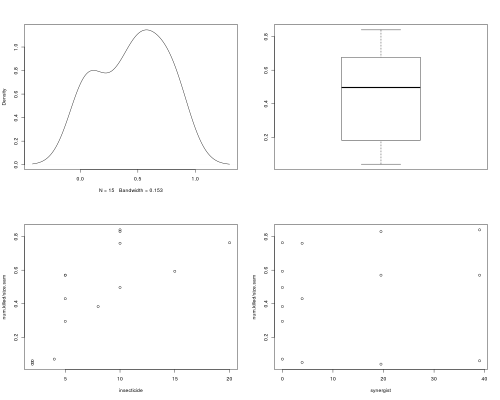
num.killed <- c(7,59,115,149,178,229,5,43,76,4,57,83,6,57,84)
size.sam <- c(1,2,3,3,3,3,rep(1,9))*100
insecticide <- c(4,5,8,10,15,20,2,5,10,2,5,10,2,5,10)
insecticide.2 <- insecticide^2
synergist <- c(rep(0,6),rep(3.9,3),rep(19.5,3),rep(39,3))

par(mfrow=c(2,2))
plot(density(num.killed/size.sam),main="")
boxplot(num.killed/size.sam)
plot(insecticide,num.killed/size.sam)
plot(synergist,num.killed/size.sam)


mean.for  <- (num.killed/size.sam) ~ insecticide  + insecticide.2
dis.for <-  ~ synergist + insecticide

res=Gammareg(mean.for,dis.for,meanlink="ide")

summary(glm((num.killed/size.sam) ~ insecticide  + insecticide.2,family=Gamma("log")))
summary(res)

# Simulation Example

X1 <- rep(1,500)
X2 <- runif(500,0,30)
X3 <- runif(500,0,15)
X4 <- runif(500,10,20)
mui <- 15 + 2*X2 + 3*X3
alphai <- exp(0.2 + 0.1*X2 + 0.3*X4)
Y <- rgamma(500,shape=alphai,scale=mui/alphai)
X <- cbind(X1,X2,X3)
Z <- cbind(X1,X2,X4)
formula.mean= Y~X2+X3
formula.shape= ~X2+X4
a=Gammareg(formula.mean,formula.shape,meanlink="ide")
summary(a)

Results


R version 3.3.1 (2016-06-21) -- "Bug in Your Hair"
Copyright (C) 2016 The R Foundation for Statistical Computing
Platform: x86_64-pc-linux-gnu (64-bit)

R is free software and comes with ABSOLUTELY NO WARRANTY.
You are welcome to redistribute it under certain conditions.
Type 'license()' or 'licence()' for distribution details.

R is a collaborative project with many contributors.
Type 'contributors()' for more information and
'citation()' on how to cite R or R packages in publications.

Type 'demo()' for some demos, 'help()' for on-line help, or
'help.start()' for an HTML browser interface to help.
Type 'q()' to quit R.

> library(Gammareg)
> png(filename="/home/ddbj/snapshot/RGM3/R_CC/result/Gammareg/Gammareg.Rd_%03d_medium.png", width=480, height=480)
> ### Name: Gammareg
> ### Title: Gammareg
> ### Aliases: Gammareg
> ### Keywords: Classic estimation Fisher Scoring joint modeling Gamma
> ###   regression Mean and shape parameters
> 
> ### ** Examples
> 
> 
> # 
> 
> num.killed <- c(7,59,115,149,178,229,5,43,76,4,57,83,6,57,84)
> size.sam <- c(1,2,3,3,3,3,rep(1,9))*100
> insecticide <- c(4,5,8,10,15,20,2,5,10,2,5,10,2,5,10)
> insecticide.2 <- insecticide^2
> synergist <- c(rep(0,6),rep(3.9,3),rep(19.5,3),rep(39,3))
> 
> par(mfrow=c(2,2))
> plot(density(num.killed/size.sam),main="")
> boxplot(num.killed/size.sam)
> plot(insecticide,num.killed/size.sam)
> plot(synergist,num.killed/size.sam)
> 
> 
> mean.for  <- (num.killed/size.sam) ~ insecticide  + insecticide.2
> dis.for <-  ~ synergist + insecticide
> 
> res=Gammareg(mean.for,dis.for,meanlink="ide")
> 
> summary(glm((num.killed/size.sam) ~ insecticide  + insecticide.2,family=Gamma("log")))

Call:
glm(formula = (num.killed/size.sam) ~ insecticide + insecticide.2, 
    family = Gamma("log"))

Deviance Residuals: 
    Min       1Q   Median       3Q      Max  
-0.8439  -0.4926  -0.1526   0.2123   0.8703  

Coefficients:
              Estimate Std. Error t value Pr(>|t|)    
(Intercept)   -3.48260    0.47761  -7.292 9.58e-06 ***
insecticide    0.52757    0.11376   4.638 0.000573 ***
insecticide.2 -0.01911    0.00546  -3.500 0.004381 ** 
---
Signif. codes:  0 '***' 0.001 '**' 0.01 '*' 0.05 '.' 0.1 ' ' 1

(Dispersion parameter for Gamma family taken to be 0.3815866)

    Null deviance: 11.9764  on 14  degrees of freedom
Residual deviance:  4.1655  on 12  degrees of freedom
AIC: -3.8819

Number of Fisher Scoring iterations: 8

> summary(res)
 
            ################################################################
            ###                  Classic Gamma Regression                ###
            ################################################################ 

 Call: 
Gammareg(formula1 = mean.for, formula2 = dis.for, meanlink = "ide")

                    Estimate    L.Intv U.Intv
beta.(Intercept)   -0.129697 -0.261399  0.002
beta.insecticide    0.119233  0.068680  0.170
beta.insecticide.2 -0.004089 -0.006540 -0.002
gamma.(Intercept)   0.439037  0.182929  0.695
gamma.synergist     0.015735  0.010504  0.021
gamma.insecticide   0.162918  0.149205  0.177

 Covariance Matrix for Beta: 
                (Intercept)   insecticide insecticide.2
(Intercept)    3.580541e-03 -1.213089e-03  5.459089e-05
insecticide   -1.213089e-03  5.275563e-04 -2.494403e-05
insecticide.2  5.459089e-05 -2.494403e-05  1.239960e-06

 Covariance Matrix for Gamma: 
              (Intercept)     synergist   insecticide
(Intercept)  0.0138168350 -2.122943e-04 -7.266857e-04
synergist   -0.0002122943  5.764239e-06  1.080063e-05
insecticide -0.0007266857  1.080063e-05  3.961207e-05

 AIC: 
[1] -577.8824

 Iteration: 
[1] 59

 Convergence: 
[1] 5.61794e-06
> 
> # Simulation Example
> 
> X1 <- rep(1,500)
> X2 <- runif(500,0,30)
> X3 <- runif(500,0,15)
> X4 <- runif(500,10,20)
> mui <- 15 + 2*X2 + 3*X3
> alphai <- exp(0.2 + 0.1*X2 + 0.3*X4)
> Y <- rgamma(500,shape=alphai,scale=mui/alphai)
> X <- cbind(X1,X2,X3)
> Z <- cbind(X1,X2,X4)
> formula.mean= Y~X2+X3
> formula.shape= ~X2+X4
> a=Gammareg(formula.mean,formula.shape,meanlink="ide")
> summary(a)
 
            ################################################################
            ###                  Classic Gamma Regression                ###
            ################################################################ 

 Call: 
Gammareg(formula1 = formula.mean, formula2 = formula.shape, meanlink = "ide")

                  Estimate  L.Intv U.Intv
beta.(Intercept)   15.3913 14.9044 15.878
beta.X2             2.0001  1.9763  2.024
beta.X3             2.9851  2.9399  3.030
gamma.(Intercept)   0.3195  0.3188  0.320
gamma.X2            0.1048  0.1048  0.105
gamma.X4            0.2866  0.2866  0.287

 Covariance Matrix for Beta: 
             (Intercept)            X2            X3
(Intercept)  0.061409236 -2.264497e-03 -2.365192e-03
X2          -0.002264497  1.460311e-04 -3.309234e-05
X3          -0.002365192 -3.309234e-05  5.280078e-04

 Covariance Matrix for Gamma: 
              (Intercept)            X2            X4
(Intercept)  1.311470e-07 -1.008708e-09 -5.763330e-09
X2          -1.008708e-09  3.772879e-11  4.617491e-12
X4          -5.763330e-09  4.617491e-12  3.084264e-10

 AIC: 
[1] 7113416

 Iteration: 
[1] 11

 Convergence: 
[1] 3.365878e-10
> 
> 
> 
> 
> 
> 
> dev.off()
null device 
          1 
>