R Graphical Manual

Browse All

Last data update: 2014.03.03

R: Saturated or K Nearest Neighbour Graph

knn.graph

R Documentation

Saturated or K Nearest Neighbour Graph

Description

Creates a kNN or saturated graph SpatialLinesDataFrame object

Usage

knn.graph(x, row.names = NULL, k = NULL, max.dist = NULL, sym = FALSE,
  long.lat = FALSE, drop.diag = FALSE)

Arguments

`x`	sp SpatialPointsDataFrame object
`row.names`	Unique row.names assigned to results
`k`	K nearest neighbours
`max.dist`	Maximum length of an edge (used for distance constraint)
`sym`	Create symmetrical graph (FALSE/TRUE)
`long.lat`	Coordinates are longitude-latitude decimal degrees (FALSE/TRUE), in which case distances are measured in kilometers
`drop.diag`	Drop diag (duplicate edges) (FALSE/TRUE)

Value

SpatialLinesDataFrame object with: i Name of column in x with FROM (origin) index j Name of column in x with TO (destination) index from_ID Name of column in x with FROM (origin) region ID to_ID Name of column in x with TO (destination) region ID length Length of each edge (line) in projection units or kilometers if long.lat = TRUE

Note

...

Author(s)

Jeffrey S. Evans <jeffrey_evans@tnc.org> and Melanie Murphy <melanie.murphy@uwyo.edu>

References

Murphy, M. A. & J.S. Evans. (in prep). "GenNetIt: gravity analysis in R for landscape genetics" Murphy M.A., R. Dezzani, D.S. Pilliod & A.S. Storfer (2010) Landscape genetics of high mountain frog metapopulations. Molecular Ecology 19(17):3634-3649

Examples

 library(sp) 
   data(ralu.site)

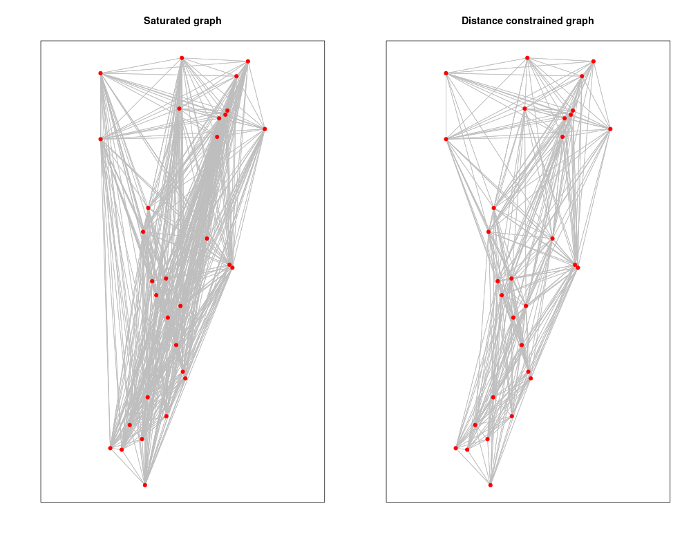
 # Saturated spatial graph
 sat.graph <- knn.graph(ralu.site, row.names=ralu.site@data[,"SiteName"])
  head(sat.graph@data)
 
 # Distanced constrained spatial graph
 dist.graph <- knn.graph(ralu.site, row.names=ralu.site@data[,"SiteName"], max.dist = 5000)

 par(mfrow=c(1,2))	
plot(sat.graph, col="grey")
  points(ralu.site, col="red", pch=20, cex=1.5)
     box()
     title("Saturated graph")	
plot(dist.graph, col="grey")
  points(ralu.site, col="red", pch=20, cex=1.5)
     box()
     title("Distance constrained graph")

Results


R version 3.3.1 (2016-06-21) -- "Bug in Your Hair"
Copyright (C) 2016 The R Foundation for Statistical Computing
Platform: x86_64-pc-linux-gnu (64-bit)

R is free software and comes with ABSOLUTELY NO WARRANTY.
You are welcome to redistribute it under certain conditions.
Type 'license()' or 'licence()' for distribution details.

R is a collaborative project with many contributors.
Type 'contributors()' for more information and
'citation()' on how to cite R or R packages in publications.

Type 'demo()' for some demos, 'help()' for on-line help, or
'help.start()' for an HTML browser interface to help.
Type 'q()' to quit R.

> library(GeNetIt)
> png(filename="/home/ddbj/snapshot/RGM3/R_CC/result/GeNetIt/knn.graph.Rd_%03d_medium.png", width=480, height=480)
> ### Name: knn.graph
> ### Title: Saturated or K Nearest Neighbour Graph
> ### Aliases: knn.graph
> 
> ### ** Examples
> 
>  library(sp) 
>    data(ralu.site)
> 
>  # Saturated spatial graph
>  sat.graph <- knn.graph(ralu.site, row.names=ralu.site@data[,"SiteName"])
>   head(sat.graph@data)
  i j      from_ID          to_ID   length
1 1 2 AirplaneLake BachelorMeadow 4126.977
2 1 3 AirplaneLake BarkingFoxLake 3110.794
3 1 4 AirplaneLake   BirdbillLake 1144.150
4 1 5 AirplaneLake        BobLake 4062.216
5 1 6 AirplaneLake      CacheLake 5726.773
6 1 7 AirplaneLake        DoeLake 6533.927
>  
>  # Distanced constrained spatial graph
>  dist.graph <- knn.graph(ralu.site, row.names=ralu.site@data[,"SiteName"], max.dist = 5000)
> 
>  par(mfrow=c(1,2))	
> plot(sat.graph, col="grey")
>   points(ralu.site, col="red", pch=20, cex=1.5)
>      box()
>      title("Saturated graph")	
> plot(dist.graph, col="grey")
>   points(ralu.site, col="red", pch=20, cex=1.5)
>      box()
>      title("Distance constrained graph")	  
> 	
> 
> 
> 
> 
> 
> dev.off()
null device 
          1 
>