R Graphical Manual

Browse All

Last data update: 2014.03.03

R: Computes (average) Idenity-by-State for a set of people and...

ibs.old

R Documentation

Computes (average) Idenity-by-State for a set of people and markers

Description

Given a set of SNPs, computes a matrix of average IBS for a group of people

Usage

ibs.old(data, snpsubset, idsubset, weight="no")

Arguments

`data`	object of `snp.data-class`
`snpsubset`	Index, character or logical vector with subset of SNPs to run analysis on. If missing, all SNPs from `data` are used for analysis.
`idsubset`	Index, character or logical vector with subset of IDs to run analysis on. If missing, all people from `data` are used for analysis.
`weight`	"no" for direct IBS computations, "freq" to weight by allelic frequency

Details

This function facilitates quality control of genomic data. E.g. people with exteremly high (close to 1) IBS may indicate duplicated samples (or twins), simply high values of IBS may indicate relatives.

When weight "freq" is used, IBS for a pair of people i and j is computed as

f_{i,j} = Σ_k frac{(x_{i,k} - p_k) * (x_{j,k} - p_k)}{(p_k * (1 - p_k))}

where k changes from 1 to N = number of SNPs GW, x_{i,k} is a genotype of ith person at the kth SNP, coded as 0, 1/2, 1 and p_k is the frequency of the "+" allele. This apparently provides an unbiased estimate of the kinship coefficient.

Only with "freq" option monomorphic SNPs are regarded as non-informative.

ibs() operation may be very lengthy for a large number of people.

Value

A (Npeople X Npeople) matrix giving average IBS (kinship) values between a pair below the diagonal and number of SNP genotype measured for both members of the pair above the diagonal.

On the diagonal, homozygosity (0.5+inbreeding) is provided.

Author(s)

Yurii Aulchenko

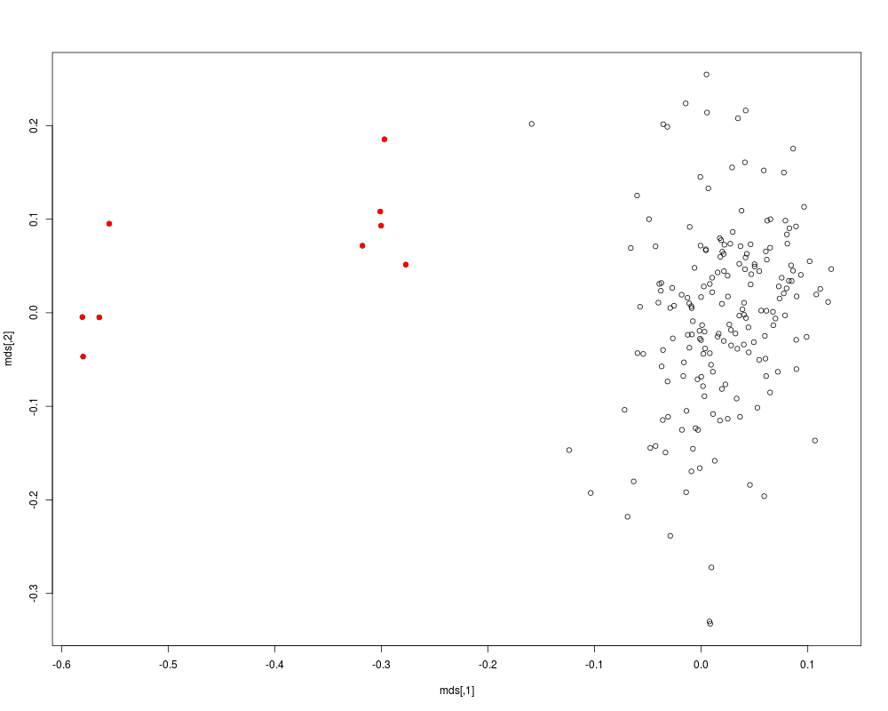
Examples

require(GenABEL.data)
data(ge03d2c)
a <- ibs(data=ge03d2c,ids=c(1:10),snps=c(1:1000))
a
# compute IBS based on a random sample of 1000 autosomal marker
a <- ibs(ge03d2c,snps=sample(ge03d2c@gtdata@snpnames[ge03d2c@gtdata@chromosome!="X"],
			1000,replace=FALSE),weight="freq")
mds <- cmdscale(as.dist(1-a))
plot(mds)
# identify smaller cluster of outliers
km <- kmeans(mds,centers=2,nstart=1000)
cl1 <- names(which(km$cluster==1))
cl2 <- names(which(km$cluster==2))
if (length(cl1) > length(cl2)) cl1 <- cl2;
cl1
# PAINT THE OUTLIERS IN RED
points(mds[cl1,],pch=19,col="red")

Results


R version 3.3.1 (2016-06-21) -- "Bug in Your Hair"
Copyright (C) 2016 The R Foundation for Statistical Computing
Platform: x86_64-pc-linux-gnu (64-bit)

R is free software and comes with ABSOLUTELY NO WARRANTY.
You are welcome to redistribute it under certain conditions.
Type 'license()' or 'licence()' for distribution details.

R is a collaborative project with many contributors.
Type 'contributors()' for more information and
'citation()' on how to cite R or R packages in publications.

Type 'demo()' for some demos, 'help()' for on-line help, or
'help.start()' for an HTML browser interface to help.
Type 'q()' to quit R.

> library(GenABEL)
Loading required package: MASS
Loading required package: GenABEL.data
> png(filename="/home/ddbj/snapshot/RGM3/R_CC/result/GenABEL/ibs.old.Rd_%03d_medium.png", width=480, height=480)
> ### Name: ibs.old
> ### Title: Computes (average) Idenity-by-State for a set of people and
> ###   markers
> ### Aliases: ibs.old
> ### Keywords: htest
> 
> ### ** Examples
> 
> require(GenABEL.data)
> data(ge03d2c)
> a <- ibs(data=ge03d2c,ids=c(1:10),snps=c(1:1000))
> a
          id199       id287       id300       id403       id415       id666
id199 0.7527750 979.0000000 980.0000000 985.0000000 978.0000000 978.0000000
id287 0.7477017   0.5015198 975.0000000 981.0000000 973.0000000 974.0000000
id300 0.7908163   0.7246154   0.7973658 981.0000000 974.0000000 974.0000000
id403 0.8000000   0.7589195   0.7900102   0.7368952 979.0000000 979.0000000
id415 0.7500000   0.7384378   0.7633470   0.7568948   0.8071066 973.0000000
id666 0.7862986   0.7766940   0.7756674   0.8094995   0.7564234   0.7497467
id689 0.7808359   0.7645855   0.7871034   0.7988798   0.8179487   0.7879098
id765 0.7762487   0.7420676   0.8781986   0.8039715   0.7564103   0.8225641
id830 0.7763562   0.7525667   0.7898253   0.8154397   0.8032956   0.7656732
id908 0.7967314   0.7622951   0.7969231   0.8384302   0.7802875   0.7738462
            id689       id765       id830       id908
id199 981.0000000 981.0000000 977.0000000 979.0000000
id287 977.0000000 977.0000000 974.0000000 976.0000000
id300 977.0000000 977.0000000 973.0000000 975.0000000
id403 982.0000000 982.0000000 978.0000000 981.0000000
id415 975.0000000 975.0000000 971.0000000 974.0000000
id666 976.0000000 975.0000000 973.0000000 975.0000000
id689   0.7350859 978.0000000 975.0000000 977.0000000
id765   0.7934560   0.7651822 975.0000000 977.0000000
id830   0.7984615   0.7984615   0.7616633 973.0000000
id908   0.8167861   0.7886387   0.8175745   0.7679838
attr(,"Var")
 [1] 0.4701928 1.4572942 0.5462274 0.3638529 0.5400270 0.3996969 0.4651762
 [8] 0.4784414 0.3620137 0.5219989
> # compute IBS based on a random sample of 1000 autosomal marker
> a <- ibs(ge03d2c,snps=sample(ge03d2c@gtdata@snpnames[ge03d2c@gtdata@chromosome!="X"],
+ 			1000,replace=FALSE),weight="freq")
> mds <- cmdscale(as.dist(1-a))
> plot(mds)
> # identify smaller cluster of outliers
> km <- kmeans(mds,centers=2,nstart=1000)
> cl1 <- names(which(km$cluster==1))
> cl2 <- names(which(km$cluster==2))
> if (length(cl1) > length(cl2)) cl1 <- cl2;
> cl1
 [1] "id287"  "id2097" "id3374" "id7715" "id6954" "id1344" "id6494" "id2136"
 [9] "id4837" "id858" 
> # PAINT THE OUTLIERS IN RED
> points(mds[cl1,],pch=19,col="red")
> 
> 
> 
> 
> 
> dev.off()
null device 
          1 
>