R Graphical Manual

Browse All

Last data update: 2014.03.03

R: Fast score test for association

qtscore

R Documentation

Fast score test for association

Description

Fast score test for association between a trait and genetic polymorphism

Usage

  qtscore(formula, data, snpsubset, idsubset, strata,
    trait.type = "gaussian", times = 1, quiet = FALSE,
    bcast = 10, clambda = TRUE, propPs = 1, details = TRUE)

Arguments

`formula`	Formula describing fixed effects to be used in analysis, e.g. y ~ a + b means that outcome (y) depends on two covariates, a and b. If no covariates used in analysis, skip the right-hand side of the equation.
`data`	An object of `gwaa.data-class`
`snpsubset`	ndex, character or logical vector with subset of SNPs to run analysis on. If missing, all SNPs from `data` are used for analysis.
`idsubset`	ndex, character or logical vector with subset of IDs to run analysis on. If missing, all people from `data/cc` are used for analysis.
`strata`	Stratification variable. If provieded, scores are computed within strata and then added up.
`trait.type`	"gaussian" or "binomial" or "guess" (later option guesses trait type)
`times`	If more than one, the number of replicas to be used in derivation of empirical genome-wide significance. See `emp.qtscore`, which calls qtscore with times>1 for details
`quiet`	do not print warning messages
`bcast`	If the argument times > 1, progress is reported once in bcast replicas
`clambda`	If inflation facot Lambda is estimated as lower then one, this parameter controls if the original P1df (clambda=TRUE) to be reported in Pc1df, or the original 1df statistics is to be multiplied onto this "deflation" factor (clambda=FALSE). If a numeric value is provided, it is used as a correction factor.
`propPs`	proportion of non-corrected P-values used to estimate the inflation factor Lambda, passed directly to the `estlambda`
`details`	when FALSE, SNP and ID names are not reported in the returned object (saves some memory). This is experimental and will be not mantained anymore as soon as we achieve better memory efficiency for storage of SNP and ID names (currently default R character data type used)

Details

When formula contains covariates, the traits is analysed using GLM and later residuals used when score test is computed for each of the SNPs in analysis. Coefficients of regression are reported for the quantitative trait.

For binary traits, odds ratios (ORs) are reportted. When adjustemnt is performed, first, "response" residuals are estimated after adjustment for covariates and scaled to [0,1]. Reported effects are approximately equal to ORs expected in logistic regression model.

With no adjustment for binary traits, 1 d.f., the test is equivalent to the Armitage test.

This is a valid function to analyse GWA data, including X chromosome. For X chromosome, stratified analysis is performed (strata=sex).

Value

Object of class scan.gwaa-class

Author(s)

Yurii Aulchenko

References

Aulchenko YS, de Koning DJ, Haley C. Genomewide rapid association using mixed model and regression: a fast and simple method for genome-wide pedigree-based quantitative trait loci association analysis. Genetics. 2007 177(1):577-85.

Amin N, van Duijn CM, Aulchenko YS. A genomic background based method for association analysis in related individuals. PLoS ONE. 2007 Dec 5;2(12):e1274.

Examples

require(GenABEL.data)
data(srdta)
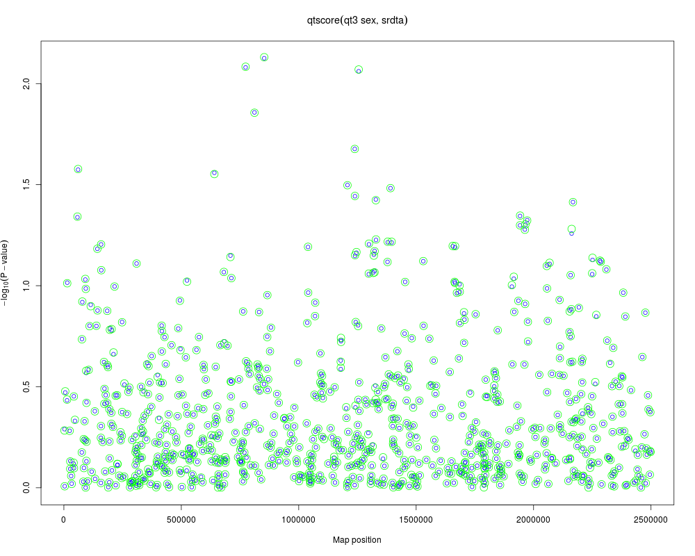
#qtscore with stratification
a <- qtscore(qt3~sex,data=srdta)
plot(a)
b <- qtscore(qt3,strata=phdata(srdta)$sex,data=srdta)
add.plot(b,col="green",cex=2)
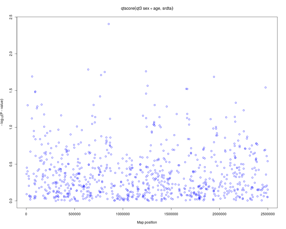
# qtscore with extra adjustment
a <- qtscore(qt3~sex+age,data=srdta)
a
plot(a)
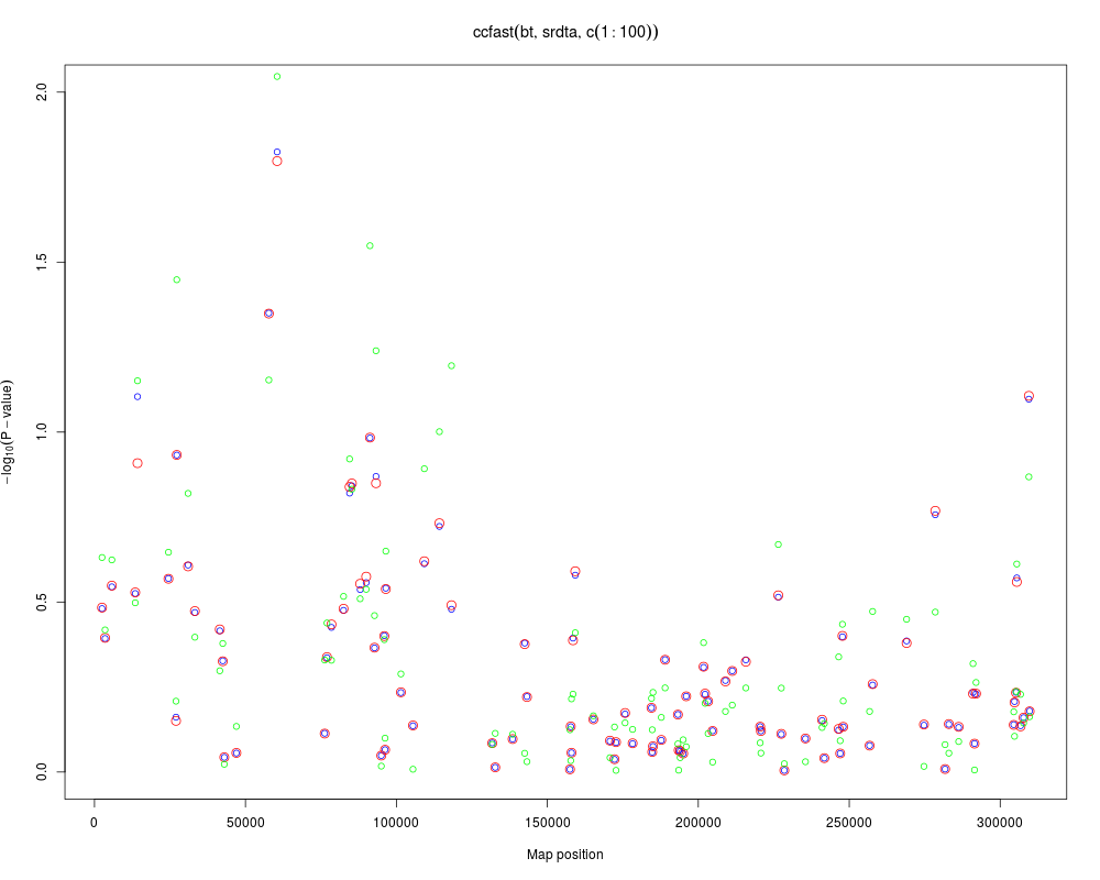
# compare results of score and chi-square test for binary trait
a1 <- ccfast("bt",data=srdta,snps=c(1:100))
a2 <- qtscore(bt,data=srdta,snps=c(1:100),trait.type="binomial")
plot(a1,ylim=c(0,2))
add.plot(a2,col="red",cex=1.5)
# the good thing about score test is that we can do adjustment...
a2 <- qtscore(bt~age+sex,data=srdta,snps=c(1:100),trait.type="binomial")
points(a2[,"Position"],-log10(a2[,"P1df"]),col="green")

Results


R version 3.3.1 (2016-06-21) -- "Bug in Your Hair"
Copyright (C) 2016 The R Foundation for Statistical Computing
Platform: x86_64-pc-linux-gnu (64-bit)

R is free software and comes with ABSOLUTELY NO WARRANTY.
You are welcome to redistribute it under certain conditions.
Type 'license()' or 'licence()' for distribution details.

R is a collaborative project with many contributors.
Type 'contributors()' for more information and
'citation()' on how to cite R or R packages in publications.

Type 'demo()' for some demos, 'help()' for on-line help, or
'help.start()' for an HTML browser interface to help.
Type 'q()' to quit R.

> library(GenABEL)
Loading required package: MASS
Loading required package: GenABEL.data
> png(filename="/home/ddbj/snapshot/RGM3/R_CC/result/GenABEL/qtscore.Rd_%03d_medium.png", width=480, height=480)
> ### Name: qtscore
> ### Title: Fast score test for association
> ### Aliases: qtscore
> ### Keywords: htest
> 
> ### ** Examples
> 
> require(GenABEL.data)
> data(srdta)
> #qtscore with stratification
> a <- qtscore(qt3~sex,data=srdta)
Warning messages:
1: In qtscore(qt3 ~ sex, data = srdta) :
  11 observations deleted due to missingness
2: In qtscore(qt3 ~ sex, data = srdta) : Lambda estimated < 1, set to 1
> plot(a)
> b <- qtscore(qt3,strata=phdata(srdta)$sex,data=srdta)
Warning messages:
1: In qtscore(qt3, strata = phdata(srdta)$sex, data = srdta) :
  11 observations deleted due to missingness
2: In qtscore(qt3, strata = phdata(srdta)$sex, data = srdta) :
  Lambda estimated < 1, set to 1
> add.plot(b,col="green",cex=2)
> # qtscore with extra adjustment
> a <- qtscore(qt3~sex+age,data=srdta)
Warning messages:
1: In qtscore(qt3 ~ sex + age, data = srdta) :
  11 observations deleted due to missingness
2: In qtscore(qt3 ~ sex + age, data = srdta) :
  Lambda estimated < 1, set to 1
> a
***** 'scan.gwaa' object *****
*** Produced with:
qtscore(formula = qt3 ~ sex + age, data = srdta)
*** Test used: gaussian 
*** no. IDs used: 2489 ( p1 p2 p3 , ... )
*** Lambda: 1 
*** Results table contains 833 rows and 9 columns
*** Output for 10 first rows is:
         N         effB    se_effB   chi2.1df       P1df        effAB
rs10  2374  0.034717185 0.04397662 0.62322553 0.42985118  0.077519239
rs18  2374 -0.007912187 0.03288150 0.05790152 0.80984395 -0.004347012
rs29  2364  0.040253046 0.04338760 0.86072851 0.35353490  0.080663818
rs65  2368  0.028201243 0.03326209 0.71884847 0.39652189  0.037455115
rs73  2375 -0.220988355 0.11279346 3.83858295 0.05008583 -0.227394158
rs114 2382  0.033892993 0.04590261 0.54518640 0.46029123  0.054671128
rs128 2380 -0.043938089 0.08948890 0.24107049 0.62343402  0.051775705
rs130 2369 -0.021537958 0.03194810 0.45448455 0.50021297  0.021241814
rs143 2366 -0.005082061 0.02961990 0.02943829 0.86377095 -0.016863497
rs150 2358 -0.006138882 0.03173327 0.03742390 0.84660453 -0.004313493
             effBB   chi2.2df      P2df
rs10  -0.186371035 3.95831922 0.1381853
rs18  -0.021599908 0.07342150 0.9639549
rs29  -0.148384469 3.77887883 0.1511565
rs65   0.062133570 0.73371540 0.6929082
rs73  -0.428076417 3.84214555 0.1464498
rs114 -0.066093408 1.30602072 0.5204766
rs128 -0.611166125 3.46117016 0.1771807
rs130 -0.019106282 0.84888653 0.6541339
rs143 -0.009027516 0.11533659 0.9439630
rs150 -0.011375984 0.03827227 0.9810458
   ...
___ Use 'results(object)' to get complete results table ___
> plot(a)
> # compare results of score and chi-square test for binary trait
> a1 <- ccfast("bt",data=srdta,snps=c(1:100))
Warning in ccfast("bt", data = srdta, snps = c(1:100)) :
  11 people (out of 2500 ) excluded as not having cc status

> a2 <- qtscore(bt,data=srdta,snps=c(1:100),trait.type="binomial")
Warning messages:
1: In qtscore(bt, data = srdta, snps = c(1:100), trait.type = "binomial") :
  11 observations deleted due to missingness
2: In qtscore(bt, data = srdta, snps = c(1:100), trait.type = "binomial") :
  Lambda estimated < 1, set to 1
> plot(a1,ylim=c(0,2))
> add.plot(a2,col="red",cex=1.5)
> # the good thing about score test is that we can do adjustment...
> a2 <- qtscore(bt~age+sex,data=srdta,snps=c(1:100),trait.type="binomial")
Warning messages:
1: In qtscore(bt ~ age + sex, data = srdta, snps = c(1:100), trait.type = "binomial") :
  11 observations deleted due to missingness
2: In qtscore(bt ~ age + sex, data = srdta, snps = c(1:100), trait.type = "binomial") :
  Lambda estimated < 1, set to 1
> points(a2[,"Position"],-log10(a2[,"P1df"]),col="green")
> 
> 
> 
> 
> 
> dev.off()
null device 
          1 
>