Univariate kernel density estimate

Description

Computes univariate kernel density estimate using Gaussian kernels which can also use non-equally spaced ordinates and adaptive bandwidths and local bandwidths

Usage

KernSec(x, xgridsize=100, xbandwidth, range.x)

Arguments

Value

returns two vectors:

Acknowledgements

Written in collaboration with A.M.Pollard <mark.pollard@rlaha.ox.ac.uk> with the financial support of the Natural Environment Research Council (NERC) grant GR3/11395

Note

Slow code suitable for visualisation and display of p.d.f where highly generalised k.p.d.fs are needed - bkde is faster when uniformly grided, single bandwidth, k.p.d.fs are required, although in the univariate case you won't notice the difference.

This function doesn't use bins as such, it calculates the density at a set of points. These points can be thought of as 'bin centres' but in reality they're not.

For version 1.10 on local kernel density estimates can now be sent, so that a vector of bandwidths can be send which is the same length as that of the observations. This will give a density which is has a unique bandwidth for each observation. Or a vector of bandwidths can be sent which is the same length as that of the number of bins. This will give a unique bandwidth for each ordinate, and is described in Wand & Jones (1995) Kernal Smoothing. It is for the user to supply this vector of bandwidths, possibly with some form of pilot estimation.

It should be noted that multi-element vectors which approximate the bin centres, can be sent rather than the extreme limits of the range; which means that the points at which the density is to be calculated need not be uniformly spaced.

If the default xbandwidth is to be used there must be at least five unique values for in the x vector. If not the function will return an error. If you don't have five unique values in the vector then send a value, or vector for xbandwidth

The number of ordinates defaults to the length of range.x if range.x is a vector of ordinates, otherwise it is xgridsize, or 100 if that isn't specified.

The option na.rm is no longer supported. The function will automatically remove NAs where appropriate and possible, and will return a warning.

Finally, the various modes of sending parameters can be mixed, ie: the extremes of the range can be sent to define the range for x, but a multi-element vector could be sent to define the ordinates in the y dimension, or, a vector could be sent to describe the bandwidth for each case in x.

Author(s)

David Lucy <d.lucy@lancaster.ac.uk> http://www.maths.lancs.ac.uk/~lucy/
Robert Aykroyd <r.g.aykroyd@leeds.ac.uk>http://www.amsta.leeds.ac.uk/~robert/

References

Lucy, D. Aykroyd, R.G. & Pollard, A.M.(2002) Non-parametric calibration for age estimation . Applied Statistics 51(2): 183-196

See Also

KernSur per density hist bkde bkde2D dpik

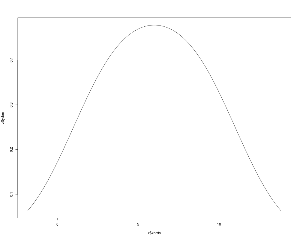
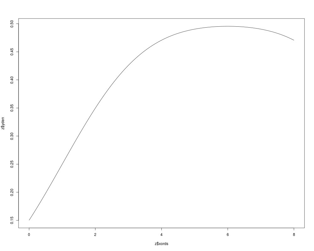
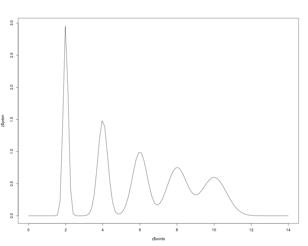
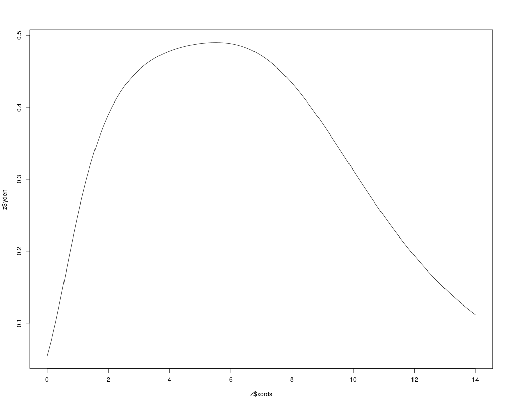
Examples

x <- c(2,4,6,8,10) 

z <- KernSec(x)				# simplest invocation
plot(z$xords, z$yden, type="l")

z <- KernSec(x, xbandwidth=2, range.x=c(0,8))
plot(z$xords, z$yden, type="l")

# local bandwidths
ords <- seq(from=0, to=14, length=100)
bands <- x/15
z <- KernSec(x, xbandwidth=bands, range.x=ords)
plot(z$xords, z$yden, type="l")         # should plot a wriggly line

bands <- seq(from=1, to=4, length=100)	# improvise a pilot estimate
z <- KernSec(x, xbandwidth=bands, range.x=ords)
plot(z$xords, z$yden, type="l") 

Results

R version 3.3.1 (2016-06-21) -- "Bug in Your Hair"
Copyright (C) 2016 The R Foundation for Statistical Computing
Platform: x86_64-pc-linux-gnu (64-bit)

R is free software and comes with ABSOLUTELY NO WARRANTY.
You are welcome to redistribute it under certain conditions.
Type 'license()' or 'licence()' for distribution details.

R is a collaborative project with many contributors.
Type 'contributors()' for more information and
'citation()' on how to cite R or R packages in publications.

Type 'demo()' for some demos, 'help()' for on-line help, or
'help.start()' for an HTML browser interface to help.
Type 'q()' to quit R.

> library(GenKern)
Loading required package: KernSmooth
KernSmooth 2.23 loaded
Copyright M. P. Wand 1997-2009
> png(filename="/home/ddbj/snapshot/RGM3/R_CC/result/GenKern/KernSec.Rd_%03d_medium.png", width=480, height=480)
> ### Name: KernSec
> ### Title: Univariate kernel density estimate
> ### Aliases: KernSec
> ### Keywords: distribution smooth
> 
> ### ** Examples
> 
> x <- c(2,4,6,8,10) 
> 
> z <- KernSec(x)				# simplest invocation
> plot(z$xords, z$yden, type="l")
> 
> z <- KernSec(x, xbandwidth=2, range.x=c(0,8))
> plot(z$xords, z$yden, type="l")
> 
> # local bandwidths
> ords <- seq(from=0, to=14, length=100)
> bands <- x/15
> z <- KernSec(x, xbandwidth=bands, range.x=ords)
> plot(z$xords, z$yden, type="l")         # should plot a wriggly line
> 
> bands <- seq(from=1, to=4, length=100)	# improvise a pilot estimate
> z <- KernSec(x, xbandwidth=bands, range.x=ords)
> plot(z$xords, z$yden, type="l") 
> 
> 
> 
> 
> 
> dev.off()
null device 
          1 
>