Supported by Dr. Osamu Ogasawara and  . . |
|
Last data update: 2014.03.03 |
Bivariate kernel density estimationDescriptionCompute bivariate kernel density estimate using five parameter Gaussian kernels which can also use non equally spaced and adaptive bandwidths UsageKernSur(x, y, xgridsize=100, ygridsize=100, correlation, xbandwidth, ybandwidth, range.x, range.y, na.rm=FALSE) Arguments
Valuereturns two vectors and a matrix:
AcknowledgementsWritten in collaboration with A.M.Pollard <mark.pollard@rlaha.ox.ac.uk> with the financial support of the Natural Environment Research Council (NERC) grant GR3/11395 NoteSlow code suitable for visualisation and display of correlated p.d.f, where highly generalised k.p.d.fs are needed - This function doesn't use bins as such, it calculates the density at a set of points in each dimension. These points can be thought of as 'bin centres' but in reality they're not. From version 1.00 onwards a number of improvements have been made: NA's are now handled semi-convincingly by dropping if required. A multi-element vector of bandwidths associated with each case can be sent for either dimension, so it is possible to accept the default, give a fixed bandwidth, or a bandwidth associated with each case. A multi-element vector of correlations can be sent, rather than a single correlation. It should be noted that if a vector is sent for correlation, or either bandwidth, they must be of the same length as the data vectors. Furthermore, vectors which approximate the bin centres, can be sent rather than the extreme limits in the range; which means that the points at which the density is to be calculated need not be uniformly spaced. Unlike If the default The number of ordinates defaults to the length of Finally, the various modes of sending parameters can be mixed, ie: the extremes of the range can be sent to define the range for Version 1.1-0 has a bugfix in that it now outputs the magnetude of the density function at the specified bi-variate points, not an approximation to the volumes. Author(s)David Lucy <d.lucy@lancaster.ac.uk> http://www.maths.lancs.ac.uk/~lucy/
ReferencesLucy, D. Aykroyd, R.G. & Pollard, A.M.(2002) Non-parametric calibration for age estimation. Applied Statistics 51(2): 183-196 See Also
Examples
x <- c(2,4,6,8,10) # make up some x-y data
y <- x
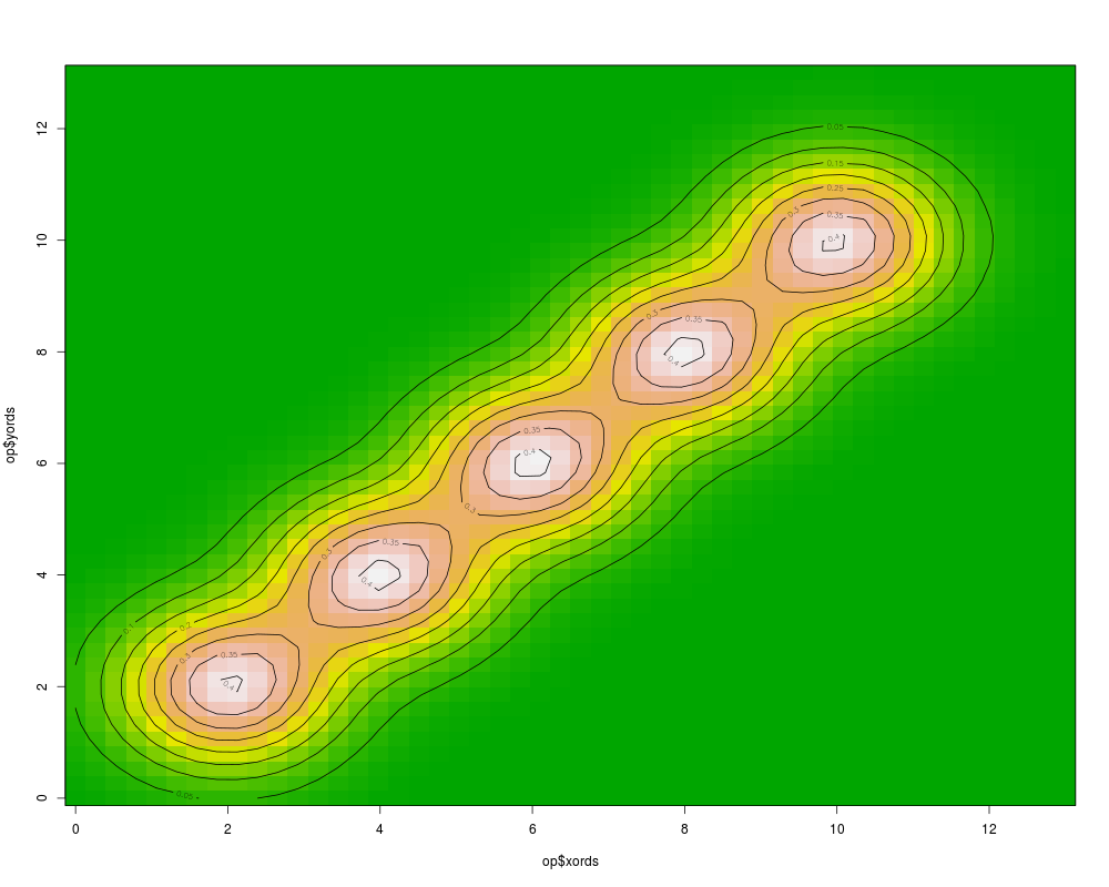
# calculate and plot a surface with zero correlation based on above data
op <- KernSur(x,y, xgridsize=50, ygridsize=50, correlation=0,
xbandwidth=1, ybandwidth=1, range.x=c(0,13), range.y=c(0,13))
image(op$xords, op$yords, op$zden, col=terrain.colors(100), axes=TRUE)
contour(op$xords, op$yords, op$zden, add=TRUE)
box()
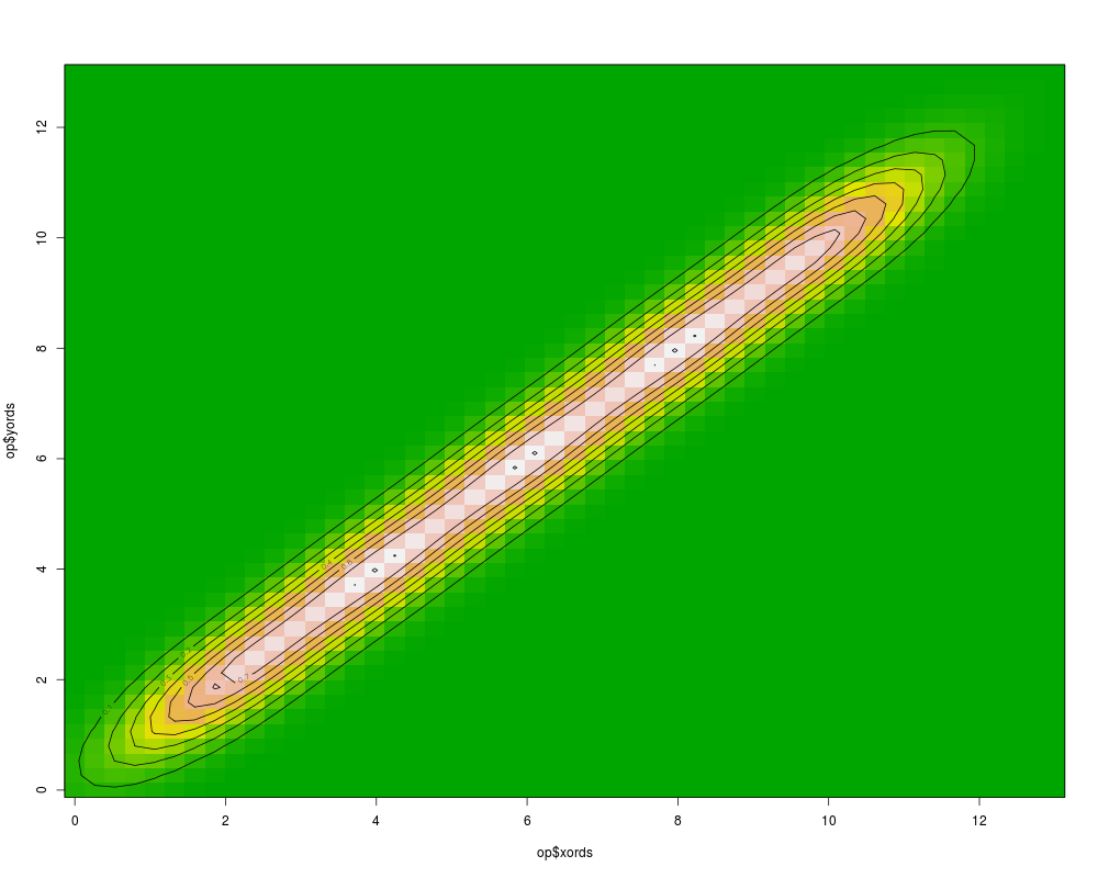
# re-calculate and re-plot the above using a 0.8 correlation
op <- KernSur(x,y, xgridsize=50, ygridsize=50, correlation=0.8,
xbandwidth=1, ybandwidth=1, range.x=c(0,13), range.y=c(0,13))
image(op$xords, op$yords, op$zden, col=terrain.colors(100), axes=TRUE)
contour(op$xords, op$yords, op$zden, add=TRUE)
box()
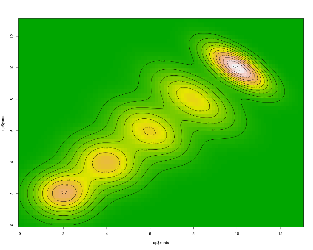
# calculate and plot a surface of the above data with an ascending
# correlation and bandwidths and a vector of equally spaced ordinates
bands <- c(1,1.1,1.2,1.3,1.0)
cors <- c(0,-0.2,-0.4,-0.6, -0.7)
rnge.x <- seq(from=0, to=13, length=100)
op <- KernSur(x,y, xgridsize=50, ygridsize=50, correlation=cors,
xbandwidth=bands, ybandwidth=bands, range.x=rnge.x, range.y=c(0,13))
image(op$xords, op$yords, op$zden, col=terrain.colors(100), axes=TRUE)
contour(op$xords, op$yords, op$zden, add=TRUE)
box()
Results
R version 3.3.1 (2016-06-21) -- "Bug in Your Hair"
Copyright (C) 2016 The R Foundation for Statistical Computing
Platform: x86_64-pc-linux-gnu (64-bit)

R is free software and comes with ABSOLUTELY NO WARRANTY.
You are welcome to redistribute it under certain conditions.
Type 'license()' or 'licence()' for distribution details.

R is a collaborative project with many contributors.
Type 'contributors()' for more information and
'citation()' on how to cite R or R packages in publications.

Type 'demo()' for some demos, 'help()' for on-line help, or
'help.start()' for an HTML browser interface to help.
Type 'q()' to quit R.

> library(GenKern)
Loading required package: KernSmooth
KernSmooth 2.23 loaded
Copyright M. P. Wand 1997-2009
> png(filename="/home/ddbj/snapshot/RGM3/R_CC/result/GenKern/KernSur.Rd_%03d_medium.png", width=480, height=480)
> ### Name: KernSur
> ### Title: Bivariate kernel density estimation
> ### Aliases: KernSur
> ### Keywords: distribution smooth
>
> ### ** Examples
>
> x <- c(2,4,6,8,10)                         # make up some x-y data
> y <- x
>
> # calculate and plot a surface with zero correlation based on above data
> op <- KernSur(x,y, xgridsize=50, ygridsize=50, correlation=0,
+         xbandwidth=1, ybandwidth=1, range.x=c(0,13), range.y=c(0,13))
> image(op$xords, op$yords, op$zden, col=terrain.colors(100), axes=TRUE)
> contour(op$xords, op$yords, op$zden, add=TRUE)
> box()
>
> # re-calculate and re-plot the above using a 0.8 correlation
> op <- KernSur(x,y, xgridsize=50, ygridsize=50, correlation=0.8,
+          xbandwidth=1, ybandwidth=1, range.x=c(0,13), range.y=c(0,13))
> image(op$xords, op$yords, op$zden, col=terrain.colors(100), axes=TRUE)
> contour(op$xords, op$yords, op$zden, add=TRUE)
> box()
>
> # calculate and plot a surface of the above data with an ascending
> # correlation and bandwidths and a vector of equally spaced ordinates
> bands <- c(1,1.1,1.2,1.3,1.0)
> cors <- c(0,-0.2,-0.4,-0.6, -0.7)
> rnge.x <- seq(from=0, to=13, length=100)
>
> op <- KernSur(x,y, xgridsize=50, ygridsize=50, correlation=cors,
+         xbandwidth=bands, ybandwidth=bands, range.x=rnge.x, range.y=c(0,13))
> image(op$xords, op$yords, op$zden, col=terrain.colors(100), axes=TRUE)
> contour(op$xords, op$yords, op$zden, add=TRUE)
> box()
>
>
>
>
>
>
> dev.off()
null device
          1
>
|