Supported by Dr. Osamu Ogasawara and  . . |
|
Last data update: 2014.03.03 |
Graphical Gaussian Models: Assess Significance of Edges (and Directions)Description
Usage
network.test.edges(r.mat, fdr=TRUE, direct=FALSE, plot=TRUE, ...)
extract.network(network.all, method.ggm=c("prob", "qval","number"),
      cutoff.ggm=0.8, method.dir=c("prob","qval","number", "all"),
      cutoff.dir=0.8, verbose=TRUE)
Arguments
DetailsFor assessing the significance of edges in the GGM
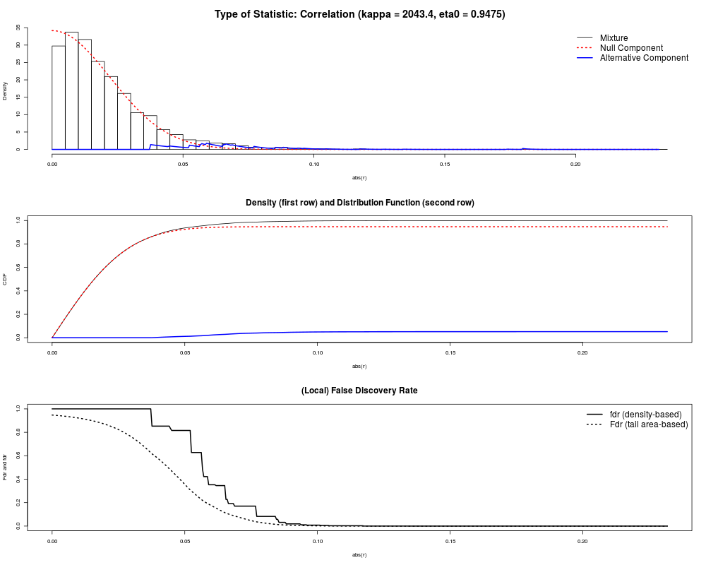
a mixture model is fitted to the partial correlations using For determining putatative directions on this GGM log-ratios of standardized partial variances re estimated, and subsequently the corresponding (local) fdr values are computed - see Opgen-Rhein and Strimmer (2007). Value
Each row in the data frame corresponds to one edge, and the rows are sorted according the absolute strength of the correlation (from strongest to weakest)
Author(s)Rainer Opgen-Rhein, Juliane Sch"afer, Korbinian Strimmer (http://strimmerlab.org). ReferencesSch"afer, J., and Strimmer, K. (2005). An empirical Bayes approach to inferring large-scale gene association networks. Bioinformatics 21:754-764. Opgen-Rhein, R., and K. Strimmer. (2007). From correlation to causation networks: a simple approximate learning algorithm and its application to high-dimensional plant gene expression data. BMC Syst. Biol. 1:37. See Also
Examples
# load GeneNet library
library("GeneNet")

# ecoli data
data(ecoli)

# estimate partial correlation matrix
inferred.pcor <- ggm.estimate.pcor(ecoli)

# p-values, q-values and posterior probabilities for each potential edge
#
test.results <- network.test.edges(inferred.pcor)

# show best 20 edges (strongest correlation)
test.results[1:20,]

# extract network containing edges with prob > 0.9 (i.e. local fdr < 0.1)
net <- extract.network(test.results, cutoff.ggm=0.9)
net

# how many are significant based on FDR cutoff Q=0.05 ?
num.significant.1 <- sum(test.results$qval <= 0.05)
test.results[1:num.significant.1,]

# how many are significant based on "local fdr" cutoff (prob > 0.9) ?
num.significant.2 <- sum(test.results$prob > 0.9)
test.results[test.results$prob > 0.9,]

# parameters of the mixture distribution used to compute p-values etc.
c <- fdrtool(sm2vec(inferred.pcor), statistic="correlation")
c$param
Results
R version 3.3.1 (2016-06-21) -- "Bug in Your Hair"
Copyright (C) 2016 The R Foundation for Statistical Computing
Platform: x86_64-pc-linux-gnu (64-bit)

R is free software and comes with ABSOLUTELY NO WARRANTY.
You are welcome to redistribute it under certain conditions.
Type 'license()' or 'licence()' for distribution details.

R is a collaborative project with many contributors.
Type 'contributors()' for more information and
'citation()' on how to cite R or R packages in publications.

Type 'demo()' for some demos, 'help()' for on-line help, or
'help.start()' for an HTML browser interface to help.
Type 'q()' to quit R.

> library(GeneNet)
Loading required package: corpcor
Loading required package: longitudinal
Loading required package: fdrtool
> png(filename="/home/ddbj/snapshot/RGM3/R_CC/result/GeneNet/network.test.edges.Rd_%03d_medium.png", width=480, height=480)
> ### Name: network.test.edges
> ### Title: Graphical Gaussian Models: Assess Significance of Edges (and
> ###   Directions)
> ### Aliases: network.test.edges extract.network
> ### Keywords: htest
>
> ### ** Examples
>
> # load GeneNet library
> library("GeneNet")
>
> # ecoli data
> data(ecoli)
>
> # estimate partial correlation matrix
> inferred.pcor <- ggm.estimate.pcor(ecoli)
Estimating optimal shrinkage intensity lambda (correlation matrix): 0.1804

>
> # p-values, q-values and posterior probabilities for each potential edge
> #
> test.results <- network.test.edges(inferred.pcor)
Estimate (local) false discovery rates (partial correlations):
Step 1... determine cutoff point
Step 2... estimate parameters of null distribution and eta0
Step 3... compute p-values and estimate empirical PDF/CDF
Step 4... compute q-values and local fdr
Step 5... prepare for plotting

>
> # show best 20 edges (strongest correlation)
> test.results[1:20,]
          pcor node1 node2         pval         qval      prob
1   0.23185664    51    53 2.220446e-16 3.612205e-13 1.0000000
2   0.22405545    52    53 2.220446e-16 3.612205e-13 1.0000000
3   0.21507824    51    52 2.220446e-16 3.612205e-13 1.0000000
4   0.17328863     7    93 3.108624e-15 3.792816e-12 0.9999945
5  -0.13418892    29    86 1.120813e-09 1.093998e-06 0.9999516
6   0.12594697    21    72 1.103837e-08 8.978569e-06 0.9998400
7   0.11956105    28    86 5.890927e-08 3.853592e-05 0.9998400
8  -0.11723897    26    80 1.060526e-07 5.816175e-05 0.9998400
9  -0.11711625    72    89 1.093655e-07 5.930502e-05 0.9972804
10  0.10658013    20    21 1.366611e-06 5.925278e-04 0.9972804
11  0.10589778    21    73 1.596860e-06 6.678431e-04 0.9972804
12  0.10478689    20    91 2.053404e-06 8.024428e-04 0.9972804
13  0.10420836     7    52 2.338383e-06 8.778608e-04 0.9944557
14  0.10236077    87    95 3.525188e-06 1.224964e-03 0.9944557
15  0.10113550    27    95 4.610445e-06 1.500048e-03 0.9920084
16  0.09928954    21    51 6.868360e-06 2.046550e-03 0.9920084
17  0.09791914    21    88 9.192376e-06 2.520617e-03 0.9920084
18  0.09719685    18    95 1.070233e-05 2.790103e-03 0.9920084
19  0.09621791    28    90 1.313008e-05 3.171818e-03 0.9920084
20  0.09619099    12    80 1.320374e-05 3.182527e-03 0.9920084
>
> # extract network containing edges with prob > 0.9 (i.e. local fdr < 0.1)
> net <- extract.network(test.results, cutoff.ggm=0.9)

Significant edges:  65
    Corresponding to  1.26 %  of possible edges
> net
          pcor node1 node2         pval         qval      prob
1   0.23185664    51    53 2.220446e-16 3.612205e-13 1.0000000
2   0.22405545    52    53 2.220446e-16 3.612205e-13 1.0000000
3   0.21507824    51    52 2.220446e-16 3.612205e-13 1.0000000
4   0.17328863     7    93 3.108624e-15 3.792816e-12 0.9999945
5  -0.13418892    29    86 1.120813e-09 1.093998e-06 0.9999516
6   0.12594697    21    72 1.103837e-08 8.978569e-06 0.9998400
7   0.11956105    28    86 5.890927e-08 3.853592e-05 0.9998400
8  -0.11723897    26    80 1.060526e-07 5.816175e-05 0.9998400
9  -0.11711625    72    89 1.093655e-07 5.930502e-05 0.9972804
10  0.10658013    20    21 1.366611e-06 5.925278e-04 0.9972804
11  0.10589778    21    73 1.596860e-06 6.678431e-04 0.9972804
12  0.10478689    20    91 2.053404e-06 8.024428e-04 0.9972804
13  0.10420836     7    52 2.338383e-06 8.778608e-04 0.9944557
14  0.10236077    87    95 3.525188e-06 1.224964e-03 0.9944557
15  0.10113550    27    95 4.610445e-06 1.500048e-03 0.9920084
16  0.09928954    21    51 6.868360e-06 2.046550e-03 0.9920084
17  0.09791914    21    88 9.192376e-06 2.520617e-03 0.9920084
18  0.09719685    18    95 1.070233e-05 2.790103e-03 0.9920084
19  0.09621791    28    90 1.313008e-05 3.171818e-03 0.9920084
20  0.09619099    12    80 1.320374e-05 3.182527e-03 0.9920084
21  0.09576091    89    95 1.443542e-05 3.354778e-03 0.9891317
22  0.09473210     7    51 1.784127e-05 3.864827e-03 0.9891317
23 -0.09386896    53    58 2.127623e-05 4.313591e-03 0.9891317
24 -0.09366615    29    83 2.217013e-05 4.421101e-03 0.9891317
25 -0.09341148    21    89 2.334321e-05 4.556948e-03 0.9810727
26 -0.09156391    49    93 3.380044e-05 5.955974e-03 0.9810727
27 -0.09150710    80    90 3.418364e-05 6.002084e-03 0.9810727
28  0.09101505     7    53 3.767967e-05 6.408104e-03 0.9810727
29  0.09050688    21    84 4.164472e-05 6.838785e-03 0.9810727
30  0.08965490    72    73 4.919367e-05 7.581868e-03 0.9810727
31 -0.08934025    29    99 5.229606e-05 7.861419e-03 0.9810727
32 -0.08906819     9    95 5.512710e-05 8.104761e-03 0.9810727
33  0.08888345     2    49 5.713146e-05 8.270675e-03 0.9810727
34  0.08850681    86    90 6.143364e-05 8.610164e-03 0.9810727
35  0.08805868    17    53 6.695172e-05 9.015178e-03 0.9810727
36  0.08790809    28    48 6.890886e-05 9.151294e-03 0.9810727
37  0.08783471    33    58 6.988213e-05 9.217600e-03 0.9682377
38 -0.08705796     7    49 8.101246e-05 1.021362e-02 0.9682377
39  0.08645033    20    46 9.086550e-05 1.102467e-02 0.9682377
40  0.08609950    48    86 9.705865e-05 1.150393e-02 0.9682377
41  0.08598769    21    52 9.911461e-05 1.165817e-02 0.9682377
42  0.08555275    32    95 1.075099e-04 1.226435e-02 0.9682377
43  0.08548231    17    51 1.089311e-04 1.236337e-02 0.9424721
44  0.08470370    80    83 1.258659e-04 1.382357e-02 0.9424721
45  0.08442510    80    82 1.325063e-04 1.437068e-02 0.9174572
46  0.08271606    80    93 1.810275e-04 1.845632e-02 0.9174572
47  0.08235175    46    91 1.933329e-04 1.941580e-02 0.9174572
48  0.08217787    25    95 1.994789e-04 1.988433e-02 0.9174572
49 -0.08170331    29    87 2.171999e-04 2.119715e-02 0.9174572
50  0.08123632    19    29 2.360717e-04 2.253606e-02 0.9174572
51  0.08101702    51    84 2.454547e-04 2.318025e-02 0.9174572
52  0.08030748    16    93 2.782643e-04 2.532796e-02 0.9174572
53  0.08006503    28    52 2.903870e-04 2.608272e-02 0.9174572
54 -0.07941656    41    80 3.252834e-04 2.814825e-02 0.9174572
55  0.07941410    54    89 3.254230e-04 2.815621e-02 0.9174572
56 -0.07934653    28    80 3.292785e-04 2.837512e-02 0.9174572
57  0.07916783    29    92 3.396803e-04 2.895702e-02 0.9174572
58 -0.07866905    17    86 3.703636e-04 3.060294e-02 0.9174572
59  0.07827749    16    29 3.962447e-04 3.191463e-02 0.9174572
60 -0.07808262    73    89 4.097453e-04 3.257290e-02 0.9174572
61  0.07766261    52    67 4.403166e-04 3.400207e-02 0.9174572
62  0.07762917    25    87 4.428397e-04 3.411638e-02 0.9174572
63 -0.07739378     9    93 4.609873e-04 3.492296e-02 0.9174572
64  0.07738885    31    80 4.613748e-04 3.493988e-02 0.9174572
65 -0.07718681    80    94 4.775137e-04 3.563445e-02 0.9174572
>
> # how many are significant based on FDR cutoff Q=0.05 ?
> num.significant.1 <- sum(test.results$qval <= 0.05)
> test.results[1:num.significant.1,]
          pcor node1 node2         pval         qval      prob
1   0.23185664    51    53 2.220446e-16 3.612205e-13 1.0000000
2   0.22405545    52    53 2.220446e-16 3.612205e-13 1.0000000
3   0.21507824    51    52 2.220446e-16 3.612205e-13 1.0000000
4   0.17328863     7    93 3.108624e-15 3.792816e-12 0.9999945
5  -0.13418892    29    86 1.120813e-09 1.093998e-06 0.9999516
6   0.12594697    21    72 1.103837e-08 8.978569e-06 0.9998400
7   0.11956105    28    86 5.890927e-08 3.853592e-05 0.9998400
8  -0.11723897    26    80 1.060526e-07 5.816175e-05 0.9998400
9  -0.11711625    72    89 1.093655e-07 5.930502e-05 0.9972804
10  0.10658013    20    21 1.366611e-06 5.925278e-04 0.9972804
11  0.10589778    21    73 1.596860e-06 6.678431e-04 0.9972804
12  0.10478689    20    91 2.053404e-06 8.024428e-04 0.9972804
13  0.10420836     7    52 2.338383e-06 8.778608e-04 0.9944557
14  0.10236077    87    95 3.525188e-06 1.224964e-03 0.9944557
15  0.10113550    27    95 4.610445e-06 1.500048e-03 0.9920084
16  0.09928954    21    51 6.868360e-06 2.046550e-03 0.9920084
17  0.09791914    21    88 9.192376e-06 2.520617e-03 0.9920084
18  0.09719685    18    95 1.070233e-05 2.790103e-03 0.9920084
19  0.09621791    28    90 1.313008e-05 3.171818e-03 0.9920084
20  0.09619099    12    80 1.320374e-05 3.182527e-03 0.9920084
21  0.09576091    89    95 1.443542e-05 3.354778e-03 0.9891317
22  0.09473210     7    51 1.784127e-05 3.864827e-03 0.9891317
23 -0.09386896    53    58 2.127623e-05 4.313591e-03 0.9891317
24 -0.09366615    29    83 2.217013e-05 4.421101e-03 0.9891317
25 -0.09341148    21    89 2.334321e-05 4.556948e-03 0.9810727
26 -0.09156391    49    93 3.380044e-05 5.955974e-03 0.9810727
27 -0.09150710    80    90 3.418364e-05 6.002084e-03 0.9810727
28  0.09101505     7    53 3.767967e-05 6.408104e-03 0.9810727
29  0.09050688    21    84 4.164472e-05 6.838785e-03 0.9810727
30  0.08965490    72    73 4.919367e-05 7.581868e-03 0.9810727
31 -0.08934025    29    99 5.229606e-05 7.861419e-03 0.9810727
32 -0.08906819     9    95 5.512710e-05 8.104761e-03 0.9810727
33  0.08888345     2    49 5.713146e-05 8.270675e-03 0.9810727
34  0.08850681    86    90 6.143364e-05 8.610164e-03 0.9810727
35  0.08805868    17    53 6.695172e-05 9.015178e-03 0.9810727
36  0.08790809    28    48 6.890886e-05 9.151294e-03 0.9810727
37  0.08783471    33    58 6.988213e-05 9.217600e-03 0.9682377
38 -0.08705796     7    49 8.101246e-05 1.021362e-02 0.9682377
39  0.08645033    20    46 9.086550e-05 1.102467e-02 0.9682377
40  0.08609950    48    86 9.705865e-05 1.150393e-02 0.9682377
41  0.08598769    21    52 9.911461e-05 1.165817e-02 0.9682377
42  0.08555275    32    95 1.075099e-04 1.226435e-02 0.9682377
43  0.08548231    17    51 1.089311e-04 1.236337e-02 0.9424721
44  0.08470370    80    83 1.258659e-04 1.382357e-02 0.9424721
45  0.08442510    80    82 1.325063e-04 1.437068e-02 0.9174572
46  0.08271606    80    93 1.810275e-04 1.845632e-02 0.9174572
47  0.08235175    46    91 1.933329e-04 1.941580e-02 0.9174572
48  0.08217787    25    95 1.994789e-04 1.988433e-02 0.9174572
49 -0.08170331    29    87 2.171999e-04 2.119715e-02 0.9174572
50  0.08123632    19    29 2.360717e-04 2.253606e-02 0.9174572
51  0.08101702    51    84 2.454547e-04 2.318025e-02 0.9174572
52  0.08030748    16    93 2.782643e-04 2.532796e-02 0.9174572
53  0.08006503    28    52 2.903870e-04 2.608272e-02 0.9174572
54 -0.07941656    41    80 3.252834e-04 2.814825e-02 0.9174572
55  0.07941410    54    89 3.254230e-04 2.815621e-02 0.9174572
56 -0.07934653    28    80 3.292785e-04 2.837512e-02 0.9174572
57  0.07916783    29    92 3.396803e-04 2.895702e-02 0.9174572
58 -0.07866905    17    86 3.703636e-04 3.060294e-02 0.9174572
59  0.07827749    16    29 3.962447e-04 3.191463e-02 0.9174572
60 -0.07808262    73    89 4.097453e-04 3.257290e-02 0.9174572
61  0.07766261    52    67 4.403166e-04 3.400207e-02 0.9174572
62  0.07762917    25    87 4.428397e-04 3.411638e-02 0.9174572
63 -0.07739378     9    93 4.609873e-04 3.492296e-02 0.9174572
64  0.07738885    31    80 4.613748e-04 3.493988e-02 0.9174572
65 -0.07718681    80    94 4.775137e-04 3.563445e-02 0.9174572
66  0.07706275    27    58 4.876832e-04 3.606179e-02 0.8297810
67 -0.07610709    16    83 5.730534e-04 4.085920e-02 0.8297810
68  0.07550557    53    84 6.337144e-04 4.406473e-02 0.8297810
>
> # how many are significant based on "local fdr" cutoff (prob > 0.9) ?
> num.significant.2 <- sum(test.results$prob > 0.9)
> test.results[test.results$prob > 0.9,]
          pcor node1 node2         pval         qval      prob
1   0.23185664    51    53 2.220446e-16 3.612205e-13 1.0000000
2   0.22405545    52    53 2.220446e-16 3.612205e-13 1.0000000
3   0.21507824    51    52 2.220446e-16 3.612205e-13 1.0000000
4   0.17328863     7    93 3.108624e-15 3.792816e-12 0.9999945
5  -0.13418892    29    86 1.120813e-09 1.093998e-06 0.9999516
6   0.12594697    21    72 1.103837e-08 8.978569e-06 0.9998400
7   0.11956105    28    86 5.890927e-08 3.853592e-05 0.9998400
8  -0.11723897    26    80 1.060526e-07 5.816175e-05 0.9998400
9  -0.11711625    72    89 1.093655e-07 5.930502e-05 0.9972804
10  0.10658013    20    21 1.366611e-06 5.925278e-04 0.9972804
11  0.10589778    21    73 1.596860e-06 6.678431e-04 0.9972804
12  0.10478689    20    91 2.053404e-06 8.024428e-04 0.9972804
13  0.10420836     7    52 2.338383e-06 8.778608e-04 0.9944557
14  0.10236077    87    95 3.525188e-06 1.224964e-03 0.9944557
15  0.10113550    27    95 4.610445e-06 1.500048e-03 0.9920084
16  0.09928954    21    51 6.868360e-06 2.046550e-03 0.9920084
17  0.09791914    21    88 9.192376e-06 2.520617e-03 0.9920084
18  0.09719685    18    95 1.070233e-05 2.790103e-03 0.9920084
19  0.09621791    28    90 1.313008e-05 3.171818e-03 0.9920084
20  0.09619099    12    80 1.320374e-05 3.182527e-03 0.9920084
21  0.09576091    89    95 1.443542e-05 3.354778e-03 0.9891317
22  0.09473210     7    51 1.784127e-05 3.864827e-03 0.9891317
23 -0.09386896    53    58 2.127623e-05 4.313591e-03 0.9891317
24 -0.09366615    29    83 2.217013e-05 4.421101e-03 0.9891317
25 -0.09341148    21    89 2.334321e-05 4.556948e-03 0.9810727
26 -0.09156391    49    93 3.380044e-05 5.955974e-03 0.9810727
27 -0.09150710    80    90 3.418364e-05 6.002084e-03 0.9810727
28  0.09101505     7    53 3.767967e-05 6.408104e-03 0.9810727
29  0.09050688    21    84 4.164472e-05 6.838785e-03 0.9810727
30  0.08965490    72    73 4.919367e-05 7.581868e-03 0.9810727
31 -0.08934025    29    99 5.229606e-05 7.861419e-03 0.9810727
32 -0.08906819     9    95 5.512710e-05 8.104761e-03 0.9810727
33  0.08888345     2    49 5.713146e-05 8.270675e-03 0.9810727
34  0.08850681    86    90 6.143364e-05 8.610164e-03 0.9810727
35  0.08805868    17    53 6.695172e-05 9.015178e-03 0.9810727
36  0.08790809    28    48 6.890886e-05 9.151294e-03 0.9810727
37  0.08783471    33    58 6.988213e-05 9.217600e-03 0.9682377
38 -0.08705796     7    49 8.101246e-05 1.021362e-02 0.9682377
39  0.08645033    20    46 9.086550e-05 1.102467e-02 0.9682377
40  0.08609950    48    86 9.705865e-05 1.150393e-02 0.9682377
41  0.08598769    21    52 9.911461e-05 1.165817e-02 0.9682377
42  0.08555275    32    95 1.075099e-04 1.226435e-02 0.9682377
43  0.08548231    17    51 1.089311e-04 1.236337e-02 0.9424721
44  0.08470370    80    83 1.258659e-04 1.382357e-02 0.9424721
45  0.08442510    80    82 1.325063e-04 1.437068e-02 0.9174572
46  0.08271606    80    93 1.810275e-04 1.845632e-02 0.9174572
47  0.08235175    46    91 1.933329e-04 1.941580e-02 0.9174572
48  0.08217787    25    95 1.994789e-04 1.988433e-02 0.9174572
49 -0.08170331    29    87 2.171999e-04 2.119715e-02 0.9174572
50  0.08123632    19    29 2.360717e-04 2.253606e-02 0.9174572
51  0.08101702    51    84 2.454547e-04 2.318025e-02 0.9174572
52  0.08030748    16    93 2.782643e-04 2.532796e-02 0.9174572
53  0.08006503    28    52 2.903870e-04 2.608272e-02 0.9174572
54 -0.07941656    41    80 3.252834e-04 2.814825e-02 0.9174572
55  0.07941410    54    89 3.254230e-04 2.815621e-02 0.9174572
56 -0.07934653    28    80 3.292785e-04 2.837512e-02 0.9174572
57  0.07916783    29    92 3.396803e-04 2.895702e-02 0.9174572
58 -0.07866905    17    86 3.703636e-04 3.060294e-02 0.9174572
59  0.07827749    16    29 3.962447e-04 3.191463e-02 0.9174572
60 -0.07808262    73    89 4.097453e-04 3.257290e-02 0.9174572
61  0.07766261    52    67 4.403166e-04 3.400207e-02 0.9174572
62  0.07762917    25    87 4.428397e-04 3.411638e-02 0.9174572
63 -0.07739378     9    93 4.609873e-04 3.492296e-02 0.9174572
64  0.07738885    31    80 4.613748e-04 3.493988e-02 0.9174572
65 -0.07718681    80    94 4.775137e-04 3.563445e-02 0.9174572
>
> # parameters of the mixture distribution used to compute p-values etc.
> c <- fdrtool(sm2vec(inferred.pcor), statistic="correlation")
Step 1... determine cutoff point
Step 2... estimate parameters of null distribution and eta0
Step 3... compute p-values and estimate empirical PDF/CDF
Step 4... compute q-values and local fdr
Step 5... prepare for plotting

> c$param
         cutoff N.cens      eta0     eta0.SE    kappa kappa.SE
[1,] 0.03553068   4352 0.9474623 0.005656465 2043.377 94.72264
>
>
>
>
>
>
> dev.off()
null device
          1
>
|