Supported by Dr. Osamu Ogasawara and  . . |
|
Last data update: 2014.03.03 |
Generalized Inverse Gaussian DistributionDescriptionDensity function, cumulative distribution function, quantile function
and random number generation for the generalized inverse Gaussian
distribution with parameter vector Usage
dgig(x, chi = 1, psi = 1, lambda = 1,
     param = c(chi, psi, lambda), KOmega = NULL)
pgig(q, chi = 1, psi = 1, lambda = 1,
     param = c(chi,psi,lambda), lower.tail = TRUE,
     ibfTol = .Machine$double.eps^(0.85), nmax = 200)
qgig(p, chi = 1, psi = 1, lambda = 1,
     param = c(chi, psi, lambda), lower.tail = TRUE,
     method = c("spline", "integrate"),
     nInterpol = 501, uniTol = 10^(-7),
     ibfTol = .Machine$double.eps^(0.85), nmax =200, ...)
rgig(n, chi = 1, psi = 1, lambda = 1,
     param = c(chi, psi, lambda))
rgig1(n, chi = 1, psi = 1, param = c(chi, psi))
ddgig(x, chi = 1, psi = 1, lambda = 1,
      param = c(chi, psi, lambda), KOmega = NULL)
Arguments
DetailsThe generalized inverse Gaussian distribution has density f(x)=(psi/chi)^{lambda/2}/ (2K_lambda(sqrt(psi chi)))x^(lambda-1) exp(-(1/2)(chi x^(-1)+psi x)) for x>0, where K_lambda() is the modified Bessel function of the third kind with order lambda. The generalized inverse Gaussian distribution is investigated in detail in J<c3><b6>rgensen (1982). Use
Calculation of quantiles using If accurate probabilities or quantiles are required, tolerances
( Generalized inverse Gaussian observations are obtained via the algorithm of Dagpunar (1989). Value
Author(s)David Scott d.scott@auckland.ac.nz, Richard Trendall, and Melanie Luen. ReferencesDagpunar, J.S. (1989). An easily implemented generalised inverse Gaussian generator. Commun. Statist. -Simula., 18, 703–710. J<c3><b6>rgensen, B. (1982). Statistical Properties of the Generalized Inverse Gaussian Distribution. Lecture Notes in Statistics, Vol. 9, Springer-Verlag, New York. Slevinsky, Richard M., and Safouhi, Hassan (2010) A recursive algorithm for the G transformation and accurate computation of incomplete Bessel functions. Appl. Numer. Math., In press. See Also
Examples
param <- c(2, 3, 1)
gigRange <- gigCalcRange(param = param, tol = 10^(-3))
par(mfrow = c(1, 2))
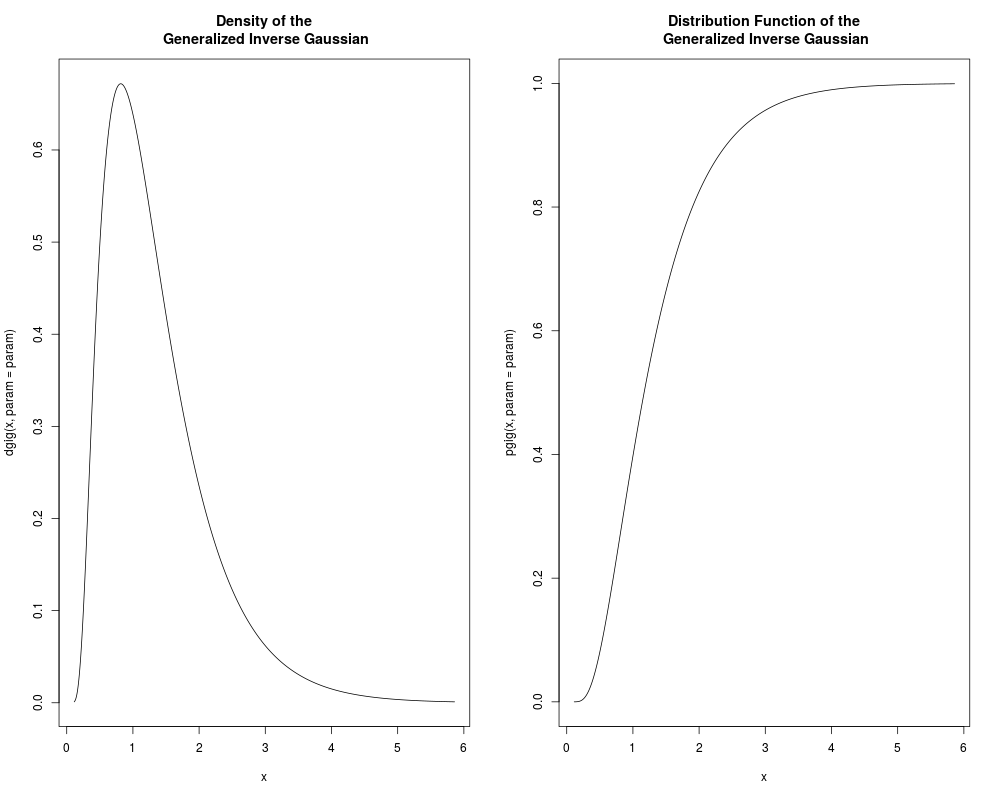
curve(dgig(x, param = param), from = gigRange[1], to = gigRange[2],
n = 1000)
title("Density of the\n Generalized Inverse Gaussian")
curve(pgig(x, param = param), from = gigRange[1], to = gigRange[2],
n = 1000)
title("Distribution Function of the\n Generalized Inverse Gaussian")
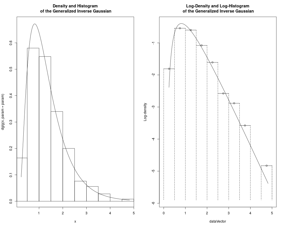
dataVector <- rgig(500, param = param)
curve(dgig(x, param = param), range(dataVector)[1], range(dataVector)[2],
n = 500)
hist(dataVector, freq = FALSE, add = TRUE)
title("Density and Histogram\n of the Generalized Inverse Gaussian")
logHist(dataVector, main =
"Log-Density and Log-Histogram\n of the Generalized Inverse Gaussian")
curve(log(dgig(x, param = param)), add = TRUE,
range(dataVector)[1], range(dataVector)[2], n = 500)
par(mfrow = c(2, 1))
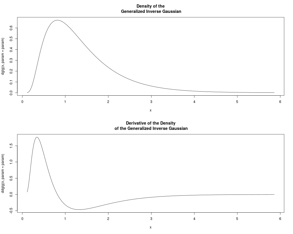
curve(dgig(x, param = param), from = gigRange[1], to = gigRange[2],
n = 1000)
title("Density of the\n Generalized Inverse Gaussian")
curve(ddgig(x, param = param), from = gigRange[1], to = gigRange[2],
n = 1000)
title("Derivative of the Density\n of the Generalized Inverse Gaussian")
Results
R version 3.3.1 (2016-06-21) -- "Bug in Your Hair"
Copyright (C) 2016 The R Foundation for Statistical Computing
Platform: x86_64-pc-linux-gnu (64-bit)

R is free software and comes with ABSOLUTELY NO WARRANTY.
You are welcome to redistribute it under certain conditions.
Type 'license()' or 'licence()' for distribution details.

R is a collaborative project with many contributors.
Type 'contributors()' for more information and
'citation()' on how to cite R or R packages in publications.

Type 'demo()' for some demos, 'help()' for on-line help, or
'help.start()' for an HTML browser interface to help.
Type 'q()' to quit R.

> library(GeneralizedHyperbolic)
Loading required package: DistributionUtils
Loading required package: RUnit
> png(filename="/home/ddbj/snapshot/RGM3/R_CC/result/GeneralizedHyperbolic/dgig.Rd_%03d_medium.png", width=480, height=480)
> ### Name: Generalized Inverse Gaussian
> ### Title: Generalized Inverse Gaussian Distribution
> ### Aliases: dgig pgig qgig rgig rgig1 ddgig
> ### Keywords: distribution
>
> ### ** Examples
>
> param <- c(2, 3, 1)
> gigRange <- gigCalcRange(param = param, tol = 10^(-3))
> par(mfrow = c(1, 2))
> curve(dgig(x, param = param), from = gigRange[1], to = gigRange[2],
+       n = 1000)
> title("Density of the\n Generalized Inverse Gaussian")
> curve(pgig(x, param = param), from = gigRange[1], to = gigRange[2],
+       n = 1000)
> title("Distribution Function of the\n Generalized Inverse Gaussian")
> dataVector <- rgig(500, param = param)
> curve(dgig(x, param = param), range(dataVector)[1], range(dataVector)[2],
+       n = 500)
> hist(dataVector, freq = FALSE, add = TRUE)
> title("Density and Histogram\n of the Generalized Inverse Gaussian")
> logHist(dataVector, main =
+         "Log-Density and Log-Histogram\n of the Generalized Inverse Gaussian")
> curve(log(dgig(x, param = param)), add = TRUE,
+       range(dataVector)[1], range(dataVector)[2], n = 500)
> par(mfrow = c(2, 1))
> curve(dgig(x, param = param), from = gigRange[1], to = gigRange[2],
+       n = 1000)
> title("Density of the\n Generalized Inverse Gaussian")
> curve(ddgig(x, param = param), from = gigRange[1], to = gigRange[2],
+       n = 1000)
> title("Derivative of the Density\n of the Generalized Inverse Gaussian")
>
>
>
>
>
> dev.off()
null device
          1
>
|