Hyperbolic Distribution

Description

Density function, distribution function, quantiles and random number generation for the hyperbolic distribution with parameter vector param. Utility routines are included for the derivative of the density function and to find suitable break points for use in determining the distribution function.

Usage

dhyperb(x, mu = 0, delta = 1, alpha = 1, beta = 0,
        param = c(mu, delta, alpha, beta))
phyperb(q, mu = 0, delta = 1, alpha = 1, beta = 0,
        param = c(mu, delta, alpha, beta),
        lower.tail = TRUE, subdivisions = 100,
        intTol = .Machine$double.eps^0.25,
        valueOnly = TRUE, ...)
qhyperb(p, mu = 0, delta = 1, alpha = 1, beta = 0,
        param = c(mu, delta, alpha, beta),
        lower.tail = TRUE, method = c("spline", "integrate"),
        nInterpol = 501, uniTol = .Machine$double.eps^0.25,
        subdivisions = 100, intTol = uniTol, ...)
rhyperb(n, mu = 0, delta = 1, alpha = 1, beta = 0,
        param = c(mu, delta, alpha, beta))
ddhyperb(x, mu = 0, delta = 1, alpha = 1, beta = 0,
         param = c(mu, delta, alpha, beta))

Arguments

Details

The hyperbolic distribution has density

f(x)=1/(2 sqrt(1+pi^2) K_1(zeta)) exp(-zeta(sqrt(1+pi^2) sqrt(1+((x-mu)/delta)^2)-pi (x-mu)/delta))

where K_1() is the modified Bessel function of the third kind with order 1.

A succinct description of the hyperbolic distribution is given in Barndorff-Nielsen and Bl<c3><a6>sild (1983). Three different possible parameterizations are described in that paper. A fourth parameterization is given in Prause (1999). All use location and scale parameters mu and delta. There are two other parameters in each case.

Use hyperbChangePars to convert from the (pi, zeta) (phi, gamma) or xi, chi) parameterizations to the (alpha, beta) parameterization used above.

Each of the functions are wrapper functions for their equivalent generalized hyperbolic counterpart. For example, dhyperb calls dghyp. See dghyp.

The hyperbolic distribution is a special case of the generalized hyperbolic distribution (Barndorff-Nielsen and Bl<c3><a6>sild (1983)). The generalized hyperbolic distribution can be represented as a particular mixture of the normal distribution where the mixing distribution is the generalized inverse Gaussian. rhyperb uses this representation to generate observations from the hyperbolic distribution. Generalized inverse Gaussian observations are obtained via the algorithm of Dagpunar (1989).

Value

dhyperb gives the density, phyperb gives the distribution function, qhyperb gives the quantile function and rhyperb generates random variates. An estimate of the accuracy of the approximation to the distribution function may be found by setting accuracy = TRUE in the call to phyperb which then returns a list with components value and error.

ddhyperb gives the derivative of dhyperb.

Author(s)

David Scott d.scott@auckland.ac.nz, Ai-Wei Lee, Jennifer Tso, Richard Trendall

References

Barndorff-Nielsen, O. and Bl<c3><a6>sild, P (1983). Hyperbolic distributions. In Encyclopedia of Statistical Sciences, eds., Johnson, N. L., Kotz, S. and Read, C. B., Vol. 3, pp. 700–707. New York: Wiley.

Dagpunar, J.S. (1989). An easily implemented generalized inverse Gaussian generator Commun. Statist. -Simula., 18, 703–710.

Prause, K. (1999) The generalized hyperbolic models: Estimation, financial derivatives and risk measurement. PhD Thesis, Mathematics Faculty, University of Freiburg.

See Also

safeIntegrate, integrate for its shortfalls, splinefun, uniroot and hyperbChangePars for changing parameters to the (alpha, beta) parameterization, dghyp for the generalized hyperbolic distribution.

Examples

param <- c(0, 2, 1, 0)
hyperbRange <- hyperbCalcRange(param = param, tol = 10^(-3))
par(mfrow = c(1, 2))
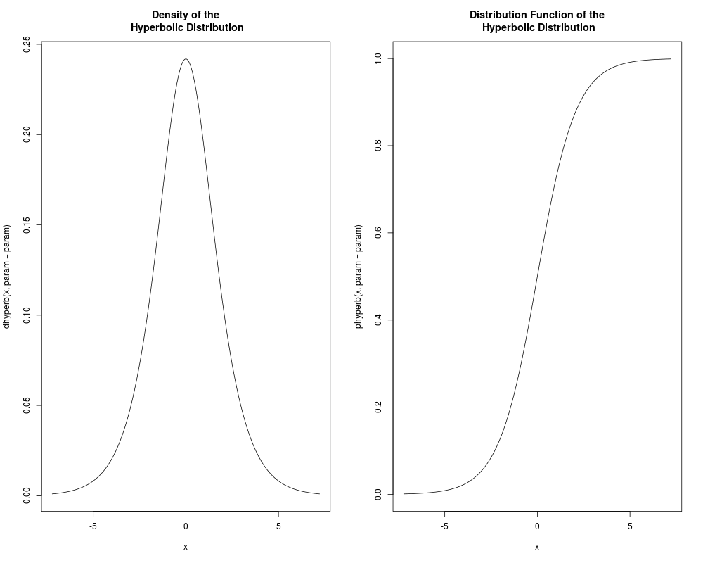
curve(dhyperb(x, param = param), from = hyperbRange[1], to = hyperbRange[2],
      n = 1000)
title("Density of the\n Hyperbolic Distribution")
curve(phyperb(x, param = param), from = hyperbRange[1], to = hyperbRange[2],
      n = 1000)
title("Distribution Function of the\n Hyperbolic Distribution")
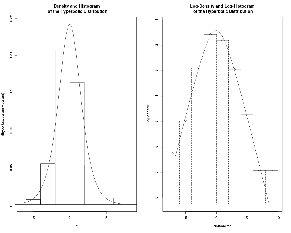
dataVector <- rhyperb(500, param = param)
curve(dhyperb(x, param = param), range(dataVector)[1], range(dataVector)[2],
      n = 500)
hist(dataVector, freq = FALSE, add =TRUE)
title("Density and Histogram\n of the Hyperbolic Distribution")
logHist(dataVector, main =
        "Log-Density and Log-Histogram\n of the Hyperbolic Distribution")
curve(log(dhyperb(x, param = param)), add = TRUE,
      range(dataVector)[1], range(dataVector)[2], n = 500)
par(mfrow = c(2, 1))
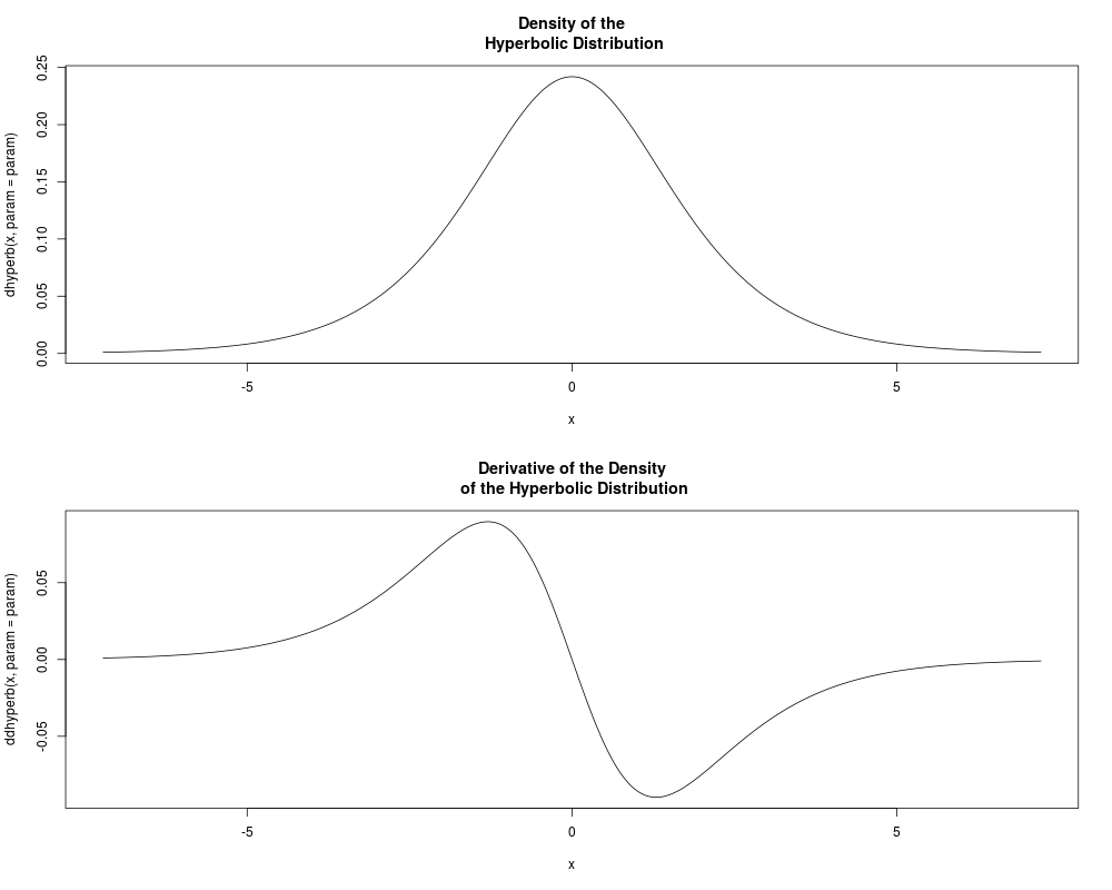
curve(dhyperb(x, param = param), from = hyperbRange[1], to = hyperbRange[2],
      n = 1000)
title("Density of the\n Hyperbolic Distribution")
curve(ddhyperb(x, param = param), from = hyperbRange[1], to = hyperbRange[2],
      n = 1000)
title("Derivative of the Density\n of the Hyperbolic Distribution")

Results

R version 3.3.1 (2016-06-21) -- "Bug in Your Hair"
Copyright (C) 2016 The R Foundation for Statistical Computing
Platform: x86_64-pc-linux-gnu (64-bit)

R is free software and comes with ABSOLUTELY NO WARRANTY.
You are welcome to redistribute it under certain conditions.
Type 'license()' or 'licence()' for distribution details.

R is a collaborative project with many contributors.
Type 'contributors()' for more information and
'citation()' on how to cite R or R packages in publications.

Type 'demo()' for some demos, 'help()' for on-line help, or
'help.start()' for an HTML browser interface to help.
Type 'q()' to quit R.

> library(GeneralizedHyperbolic)
Loading required package: DistributionUtils
Loading required package: RUnit
> png(filename="/home/ddbj/snapshot/RGM3/R_CC/result/GeneralizedHyperbolic/dhyperb.Rd_%03d_medium.png", width=480, height=480)
> ### Name: Hyperbolic
> ### Title: Hyperbolic Distribution
> ### Aliases: dhyperb phyperb qhyperb rhyperb ddhyperb
> ### Keywords: distribution
> 
> ### ** Examples
> 
> param <- c(0, 2, 1, 0)
> hyperbRange <- hyperbCalcRange(param = param, tol = 10^(-3))
> par(mfrow = c(1, 2))
> curve(dhyperb(x, param = param), from = hyperbRange[1], to = hyperbRange[2],
+       n = 1000)
> title("Density of the\n Hyperbolic Distribution")
> curve(phyperb(x, param = param), from = hyperbRange[1], to = hyperbRange[2],
+       n = 1000)
> title("Distribution Function of the\n Hyperbolic Distribution")
> dataVector <- rhyperb(500, param = param)
> curve(dhyperb(x, param = param), range(dataVector)[1], range(dataVector)[2],
+       n = 500)
> hist(dataVector, freq = FALSE, add =TRUE)
> title("Density and Histogram\n of the Hyperbolic Distribution")
> logHist(dataVector, main =
+         "Log-Density and Log-Histogram\n of the Hyperbolic Distribution")
> curve(log(dhyperb(x, param = param)), add = TRUE,
+       range(dataVector)[1], range(dataVector)[2], n = 500)
> par(mfrow = c(2, 1))
> curve(dhyperb(x, param = param), from = hyperbRange[1], to = hyperbRange[2],
+       n = 1000)
> title("Density of the\n Hyperbolic Distribution")
> curve(ddhyperb(x, param = param), from = hyperbRange[1], to = hyperbRange[2],
+       n = 1000)
> title("Derivative of the Density\n of the Hyperbolic Distribution")
> 
> 
> 
> 
> 
> dev.off()
null device 
          1 
>