Skew-Laplace Distribution

Description

Density function, distribution function, quantiles and random number generation for the skew-Laplace distribution.

Usage

dskewlap(x, mu = 0, alpha = 1, beta = 1,
         param = c(mu, alpha, beta), logPars = FALSE)
pskewlap(q, mu = 0, alpha = 1, beta = 1,
         param = c(mu, alpha, beta))
qskewlap(p, mu = 0, alpha = 1, beta = 1,
         param = c(mu, alpha, beta))
rskewlap(n, mu = 0, alpha = 1, beta = 1,
         param = c(mu, alpha, beta))

Arguments

.

Details

The central skew-Laplace has mode zero, and is a mixture of a (negative) exponential distribution with mean beta, and the negative of an exponential distribution with mean alpha. The weights of the positive and negative components are proportional to their means.

The general skew-Laplace distribution is a shifted central skew-Laplace distribution, where the mode is given by mu.

The density is given by:

f(x)=(1/(alpha+beta)) e^((x - mu)/alpha)

for x <= mu, and

f(x)=(1/(alpha+beta)) e^(-(x - mu)/beta)

for x >= mu

Value

dskewlap gives the density, pskewlap gives the distribution function, qskewlap gives the quantile function and rskewlap generates random variates. The distribution function is obtained by elementary integration of the density function. Random variates are generated from exponential observations using the characterization of the skew-Laplace as a mixture of exponential observations.

Author(s)

David Scott d.scott@auckland.ac.nz, Ai-Wei Lee, Richard Trendall

References

Fieller, N. J., Flenley, E. C. and Olbricht, W. (1992) Statistics of particle size data. Appl. Statist., 41, 127–146.

See Also

hyperbFitStart

Examples

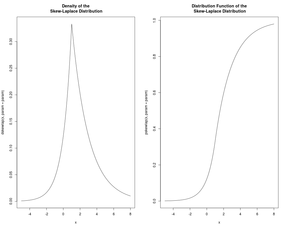
param <- c(1, 1, 2)
par(mfrow = c(1, 2))
curve(dskewlap(x, param = param), from = -5, to = 8, n = 1000)
title("Density of the\n Skew-Laplace Distribution")
curve(pskewlap(x, param = param), from = -5, to = 8, n = 1000)
title("Distribution Function of the\n Skew-Laplace Distribution")
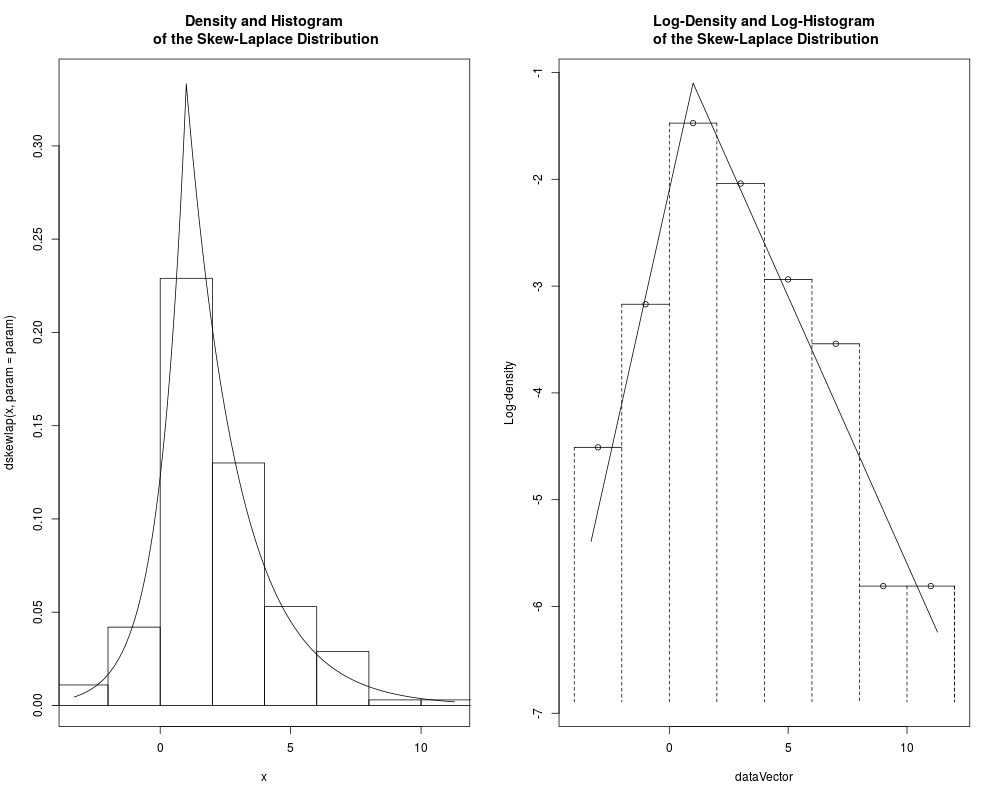
dataVector <- rskewlap(500, param = param)
curve(dskewlap(x, param = param), range(dataVector)[1], range(dataVector)[2],
      n = 500)
hist(dataVector, freq = FALSE, add = TRUE)
title("Density and Histogram\n of the Skew-Laplace Distribution")
logHist(dataVector, main =
        "Log-Density and Log-Histogram\n of the Skew-Laplace Distribution")
curve(log(dskewlap(x, param = param)), add = TRUE,
      range(dataVector)[1], range(dataVector)[2], n = 500)

Results

R version 3.3.1 (2016-06-21) -- "Bug in Your Hair"
Copyright (C) 2016 The R Foundation for Statistical Computing
Platform: x86_64-pc-linux-gnu (64-bit)

R is free software and comes with ABSOLUTELY NO WARRANTY.
You are welcome to redistribute it under certain conditions.
Type 'license()' or 'licence()' for distribution details.

R is a collaborative project with many contributors.
Type 'contributors()' for more information and
'citation()' on how to cite R or R packages in publications.

Type 'demo()' for some demos, 'help()' for on-line help, or
'help.start()' for an HTML browser interface to help.
Type 'q()' to quit R.

> library(GeneralizedHyperbolic)
Loading required package: DistributionUtils
Loading required package: RUnit
> png(filename="/home/ddbj/snapshot/RGM3/R_CC/result/GeneralizedHyperbolic/dskewlap.Rd_%03d_medium.png", width=480, height=480)
> ### Name: SkewLaplace
> ### Title: Skew-Laplace Distribution
> ### Aliases: dskewlap pskewlap qskewlap rskewlap
> ### Keywords: distribution
> 
> ### ** Examples
> 
> param <- c(1, 1, 2)
> par(mfrow = c(1, 2))
> curve(dskewlap(x, param = param), from = -5, to = 8, n = 1000)
> title("Density of the\n Skew-Laplace Distribution")
> curve(pskewlap(x, param = param), from = -5, to = 8, n = 1000)
> title("Distribution Function of the\n Skew-Laplace Distribution")
> dataVector <- rskewlap(500, param = param)
> curve(dskewlap(x, param = param), range(dataVector)[1], range(dataVector)[2],
+       n = 500)
> hist(dataVector, freq = FALSE, add = TRUE)
> title("Density and Histogram\n of the Skew-Laplace Distribution")
> logHist(dataVector, main =
+         "Log-Density and Log-Histogram\n of the Skew-Laplace Distribution")
> curve(log(dskewlap(x, param = param)), add = TRUE,
+       range(dataVector)[1], range(dataVector)[2], n = 500)
> 
> 
> 
> 
> 
> dev.off()
null device 
          1 
>