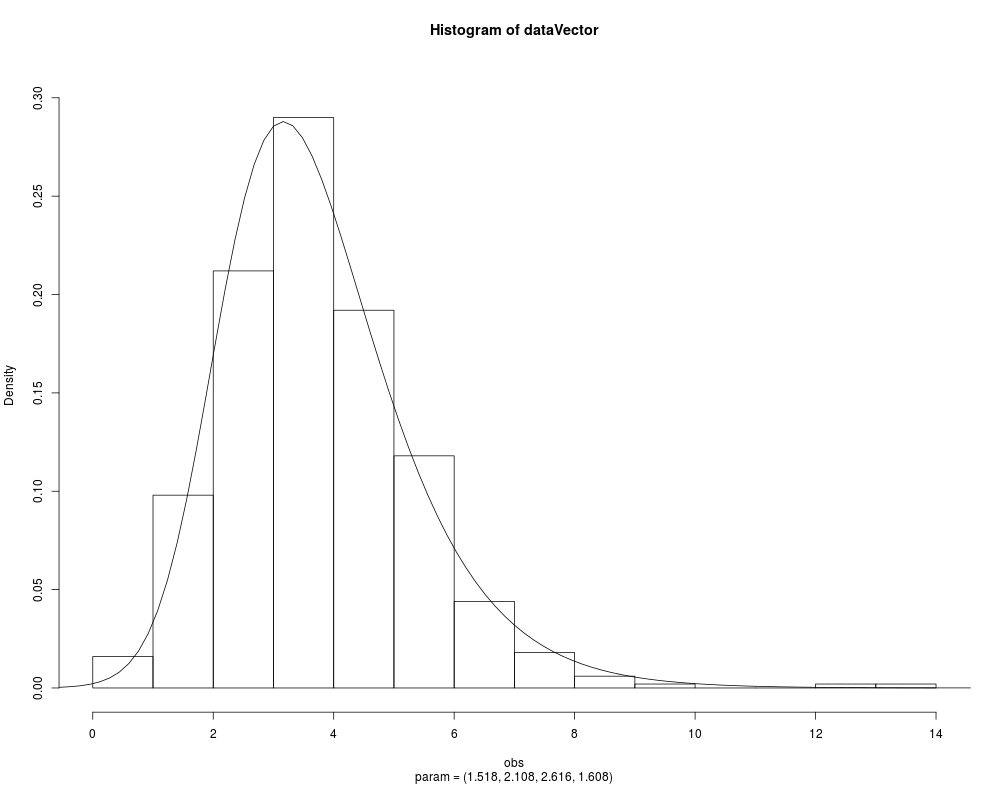
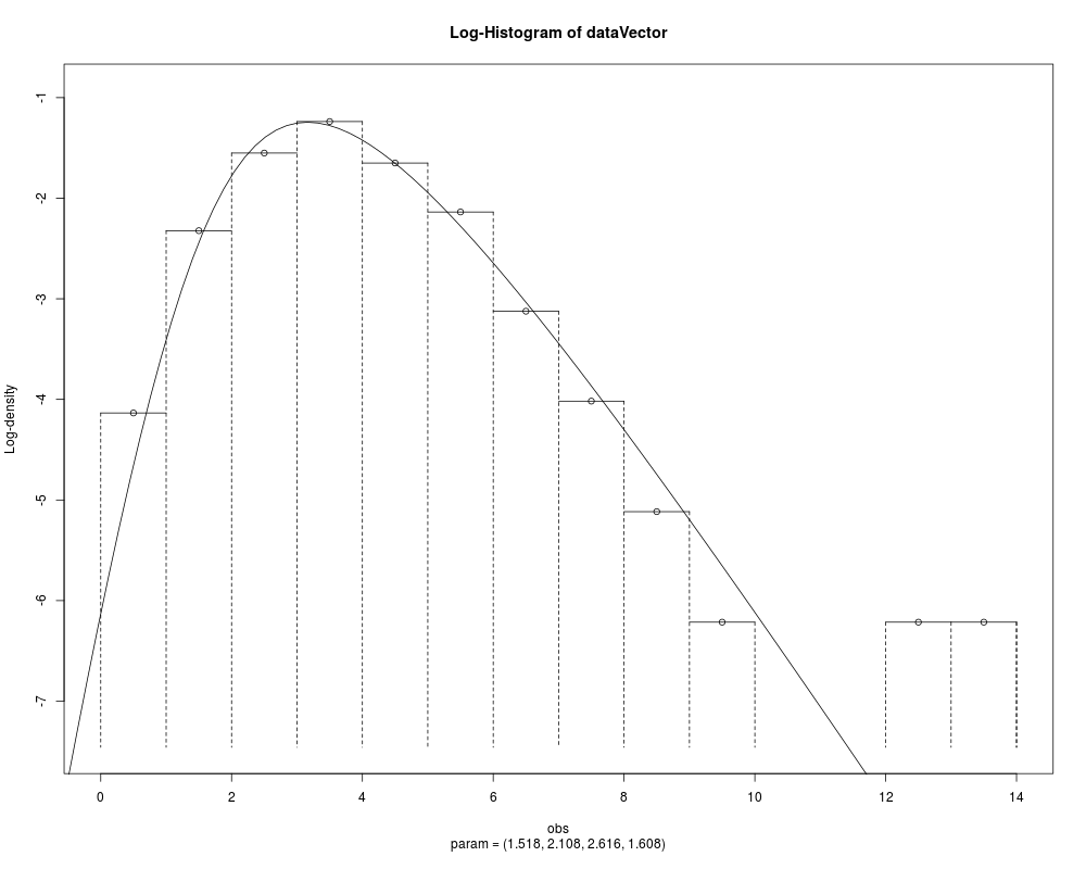
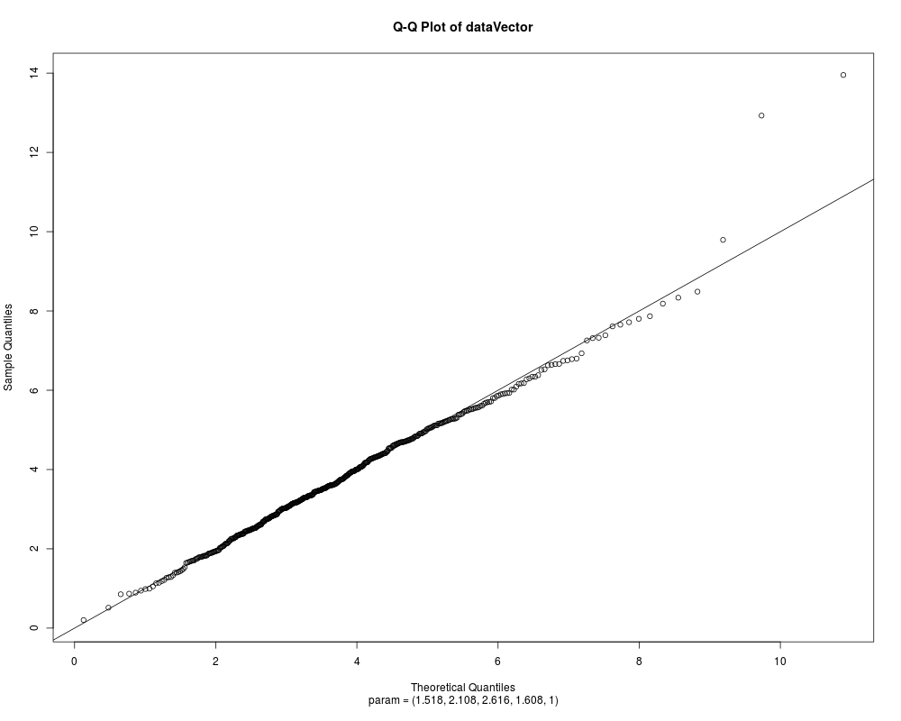
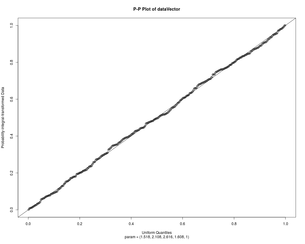
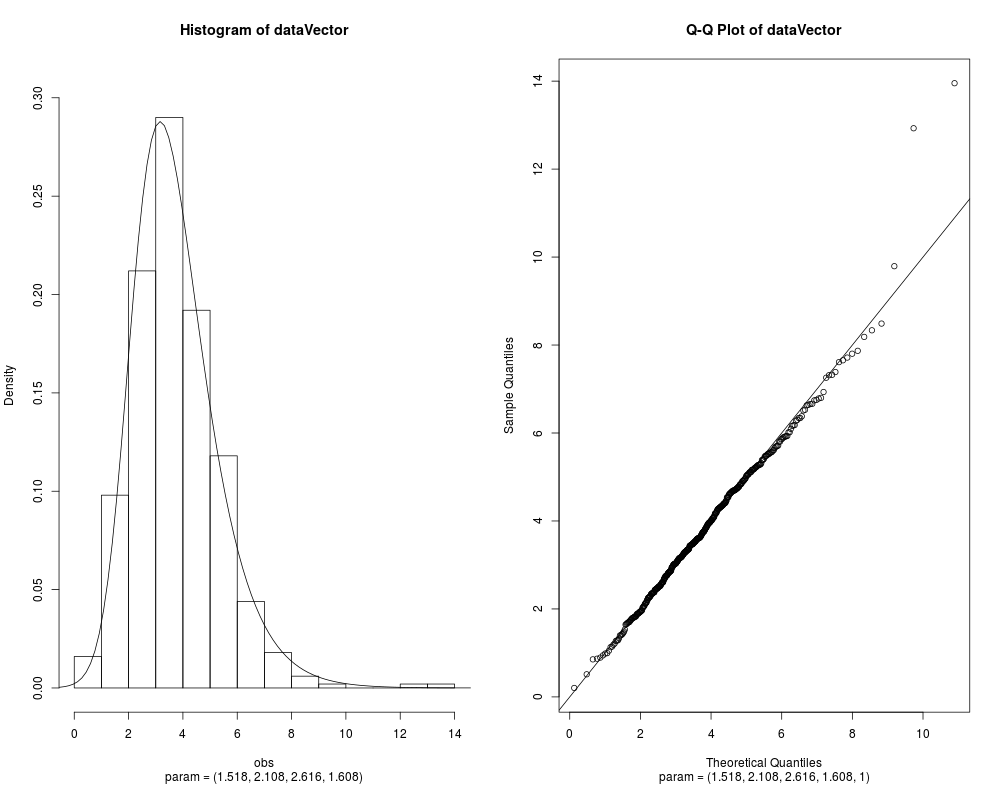
Fit the Hyperbolic Distribution to Data

Description

Fits a hyperbolic distribution to data. Displays the histogram, log-histogram (both with fitted densities), Q-Q plot and P-P plot for the fit which has the maximum likelihood.

Usage

  hyperbFit(x, freq = NULL, paramStart = NULL,
            startMethod = c("Nelder-Mead","BFGS"),
            startValues = c("BN","US","FN","SL","MoM"),
            criterion = "MLE",
            method = c("Nelder-Mead","BFGS","nlm",
                       "L-BFGS-B","nlminb","constrOptim"),
            plots = FALSE, printOut = FALSE,
            controlBFGS = list(maxit = 200),
            controlNM = list(maxit = 1000), maxitNLM = 1500,
            controlLBFGSB = list(maxit = 200),
            controlNLMINB = list(),
            controlCO = list(), ...)

  ## S3 method for class 'hyperbFit'
print(x,
        digits = max(3, getOption("digits") - 3), ...)

  ## S3 method for class 'hyperbFit'
plot(x, which = 1:4,
     plotTitles = paste(c("Histogram of ","Log-Histogram of ",
                        "Q-Q Plot of ","P-P Plot of "), x$obsName,
                        sep = ""),
     ask = prod(par("mfcol")) < length(which) & dev.interactive(), ...)

  ## S3 method for class 'hyperbFit'
coef(object, ...)

  ## S3 method for class 'hyperbFit'
vcov(object, ...)

Arguments

Details

startMethod can be either "BFGS" or "Nelder-Mead".

startValues can be one of the following:

• "US"User-supplied.

• "BN"Based on Barndorff-Nielsen (1977).

• "FN"A fitted normal distribution.

• "SL"Based on a fitted skew-Laplace distribution.

• "MoM"Method of moments.

For the details concerning the use of paramStart, startMethod, and startValues, see hyperbFitStart.

The six optimisation methods currently available are:

• "BFGS"Uses the quasi-Newton method "BFGS" as documented in optim.

• "Nelder-Mead"Uses an implementation of the Nelder and Mead method as documented in optim.

• "nlm"Uses the nlm function in R.

• "L-BFGS-B"Uses the quasi-Newton method with box constraints "L-BFGS-B" as documented in optim.

• "nlminb"Uses the nlminb function in R.

• "constrOptim"Uses the constrOptim function in R.

For details of how to pass control information for optimisation using optim, nlm, nlminb and constrOptim, see optim, nlm, nlminb and constrOptim.

When method = "nlm" is used, warnings may be produced. These do not appear to be a problem.

Value

hyperbFit returns a list with components:

Author(s)

David Scott d.scott@auckland.ac.nz, Ai-Wei Lee, Jennifer Tso, Richard Trendall, Thomas Tran, Christine Yang Dong

References

Barndorff-Nielsen, O. (1977) Exponentially decreasing distributions for the logarithm of particle size, Proc. Roy. Soc. Lond., A353, 401–419.

Fieller, N. J., Flenley, E. C. and Olbricht, W. (1992) Statistics of particle size data. Appl. Statist., 41, 127–146.

See Also

optim, nlm, nlminb, constrOptim, par, hist, logHist, qqhyperb, pphyperb, dskewlap and hyperbFitStart.

Examples

param <- c(2, 2, 2, 1)
dataVector <- rhyperb(500, param = param)
## See how well hyperbFit works
hyperbFit(dataVector)
hyperbFit(dataVector, plots = TRUE)
fit <- hyperbFit(dataVector)
par(mfrow = c(1, 2))
plot(fit, which = c(1, 3))

## Use nlm instead of default
hyperbFit(dataVector, method = "nlm")

Results

R version 3.3.1 (2016-06-21) -- "Bug in Your Hair"
Copyright (C) 2016 The R Foundation for Statistical Computing
Platform: x86_64-pc-linux-gnu (64-bit)

R is free software and comes with ABSOLUTELY NO WARRANTY.
You are welcome to redistribute it under certain conditions.
Type 'license()' or 'licence()' for distribution details.

R is a collaborative project with many contributors.
Type 'contributors()' for more information and
'citation()' on how to cite R or R packages in publications.

Type 'demo()' for some demos, 'help()' for on-line help, or
'help.start()' for an HTML browser interface to help.
Type 'q()' to quit R.

> library(GeneralizedHyperbolic)
Loading required package: DistributionUtils
Loading required package: RUnit
> png(filename="/home/ddbj/snapshot/RGM3/R_CC/result/GeneralizedHyperbolic/hyperbFit.Rd_%03d_medium.png", width=480, height=480)
> ### Name: hyperbFit
> ### Title: Fit the Hyperbolic Distribution to Data
> ### Aliases: hyperbFit print.hyperbFit plot.hyperbFit coef.hyperbFit
> ###   vcov.hyperbFit
> ### Keywords: distribution
> 
> ### ** Examples
> 
> param <- c(2, 2, 2, 1)
> dataVector <- rhyperb(500, param = param)
> ## See how well hyperbFit works
> hyperbFit(dataVector)

Data:      dataVector 
Parameter estimates:
   mu  delta  alpha   beta  
1.655  1.881  2.505  1.484  
Likelihood:         -883.7581 
criterion :         MLE 
Method:             Nelder-Mead 
Convergence code:   0 
Iterations:         237 
> hyperbFit(dataVector, plots = TRUE)

Data:      dataVector 
Parameter estimates:
   mu  delta  alpha   beta  
1.655  1.881  2.505  1.484  
Likelihood:         -883.7581 
criterion :         MLE 
Method:             Nelder-Mead 
Convergence code:   0 
Iterations:         237 
> fit <- hyperbFit(dataVector)
> par(mfrow = c(1, 2))
> plot(fit, which = c(1, 3))
> 
> ## Use nlm instead of default
> hyperbFit(dataVector, method = "nlm")

Data:      dataVector 
Parameter estimates:
   mu  delta  alpha   beta  
1.655  1.881  2.503  1.483  
Likelihood:         -883.758 
criterion :         MLE 
Method:             nlm 
Convergence code:   1 
Iterations:         27 
Warning message:
In nlm(llfunc, paramStart, iterlim = maxitNLM, ...) :
  NA/Inf replaced by maximum positive value
> 
> 
> 
> 
> 
> 
> dev.off()
null device 
          1 
>