R Graphical Manual

Browse All

Last data update: 2014.03.03

R: Generalized Hyperbolic Quantile-Quantile and Percent-Percent...

GeneralizedHyperbolicPlots

R Documentation

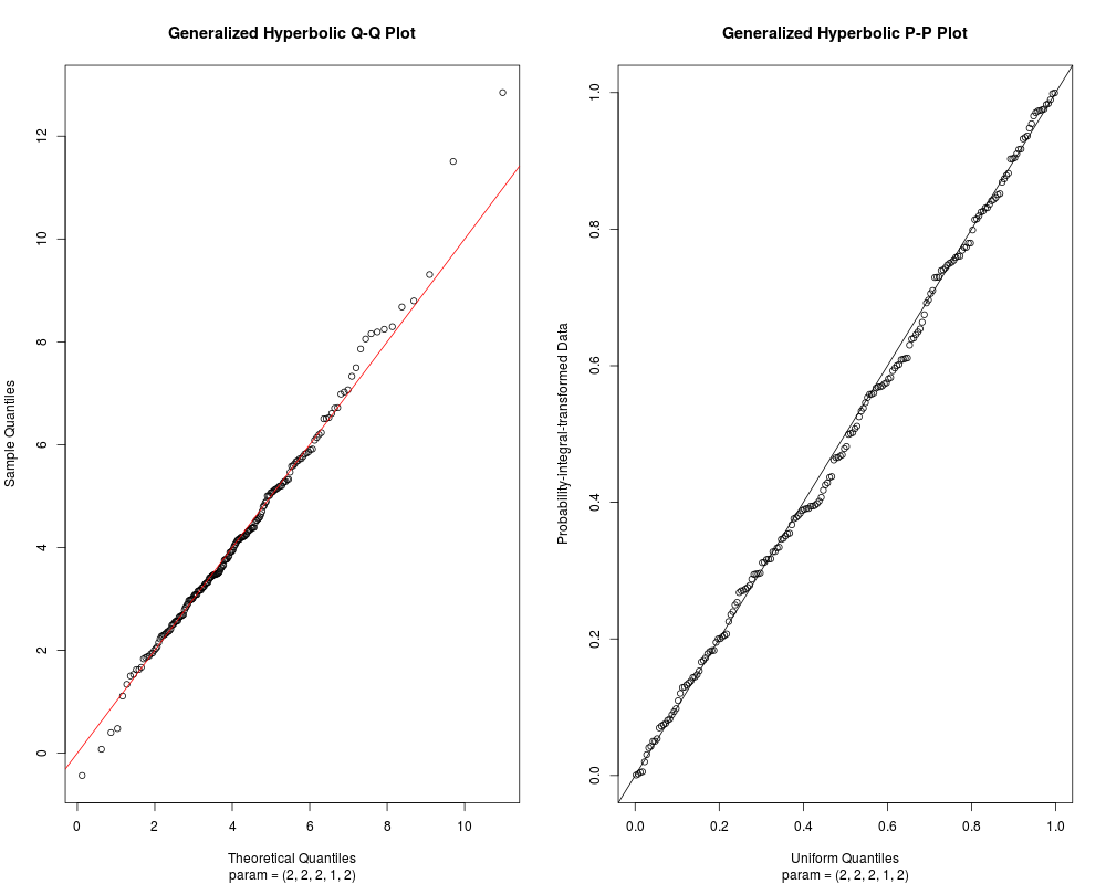
Generalized Hyperbolic Quantile-Quantile and Percent-Percent Plots

Description

qqghyp produces a generalized hyperbolic Q-Q plot of the values in y.

ppghyp produces a generalized hyperbolic P-P (percent-percent) or probability plot of the values in y.

Graphical parameters may be given as arguments to qqghyp, and ppghyp.

Usage

qqghyp(y, mu = 0, delta = 1, alpha = 1, beta = 0, lambda = 1,
       param = c(mu, delta, alpha, beta, lambda),
       main = "Generalized Hyperbolic Q-Q Plot",
       xlab = "Theoretical Quantiles",
       ylab = "Sample Quantiles",
       plot.it = TRUE, line = TRUE, ...)

ppghyp(y, mu = 0, delta = 1, alpha = 1, beta = 0, lambda = 1,
       param = c(mu, delta, alpha, beta, lambda),
       main = "Generalized Hyperbolic P-P Plot",
       xlab = "Uniform Quantiles",
       ylab = "Probability-integral-transformed Data",
       plot.it = TRUE, line = TRUE, ...)

Arguments

`y`	The data sample.
`mu`	mu is the location parameter. By default this is set to 0.
`delta`	delta is the scale parameter of the distribution. A default value of 1 has been set.
`alpha`	alpha is the tail parameter, with a default value of 1.
`beta`	beta is the skewness parameter, by default this is 0.
`lambda`	lambda is the shape parameter and dictates the shape that the distribution shall take. Default value is 1.
`param`	Parameters of the generalized hyperbolic distribution.
`xlab, ylab, main`	Plot labels.
`plot.it`	Logical. Should the result be plotted?
`line`	Add line through origin with unit slope.
`...`	Further graphical parameters.

Value

For qqghyp and ppghyp, a list with components:

`x`	The x coordinates of the points that are to be plotted.
`y`	The y coordinates of the points that are to be plotted.

References

Wilk, M. B. and Gnanadesikan, R. (1968) Probability plotting methods for the analysis of data. Biometrika. 55, 1–17.

Examples

par(mfrow = c(1, 2))
y <- rghyp(200, param = c(2, 2, 2, 1, 2))
qqghyp(y, param = c(2, 2, 2, 1, 2), line = FALSE)
abline(0, 1, col = 2)
ppghyp(y, param = c(2, 2, 2, 1, 2))

Results


R version 3.3.1 (2016-06-21) -- "Bug in Your Hair"
Copyright (C) 2016 The R Foundation for Statistical Computing
Platform: x86_64-pc-linux-gnu (64-bit)

R is free software and comes with ABSOLUTELY NO WARRANTY.
You are welcome to redistribute it under certain conditions.
Type 'license()' or 'licence()' for distribution details.

R is a collaborative project with many contributors.
Type 'contributors()' for more information and
'citation()' on how to cite R or R packages in publications.

Type 'demo()' for some demos, 'help()' for on-line help, or
'help.start()' for an HTML browser interface to help.
Type 'q()' to quit R.

> library(GeneralizedHyperbolic)
Loading required package: DistributionUtils
Loading required package: RUnit
> png(filename="/home/ddbj/snapshot/RGM3/R_CC/result/GeneralizedHyperbolic/qqghyp.Rd_%03d_medium.png", width=480, height=480)
> ### Name: GeneralizedHyperbolicPlots
> ### Title: Generalized Hyperbolic Quantile-Quantile and Percent-Percent
> ###   Plots
> ### Aliases: qqghyp ppghyp
> ### Keywords: hplot distribution
> 
> ### ** Examples
> 
> par(mfrow = c(1, 2))
> y <- rghyp(200, param = c(2, 2, 2, 1, 2))
> qqghyp(y, param = c(2, 2, 2, 1, 2), line = FALSE)
> abline(0, 1, col = 2)
> ppghyp(y, param = c(2, 2, 2, 1, 2))
> 
> 
> 
> 
> 
> dev.off()
null device 
          1 
>