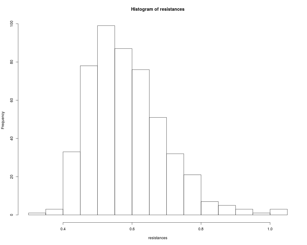
Resistance of One-half-ohm Resistors

Description

This data set gives the resistance in ohms of 500 nominally one-half-ohm resistors, presented in Hahn and Shapiro (1967). Summary data giving the frequency of observations in 28 intervals.

Usage

data(resistors)

Format

The resistors data frame has 28 rows and 2 columns.

Source

Hahn, Gerald J. and Shapiro, Samuel S. (1967) Statistical Models in Engineering. New York: Wiley, page 207.

References

Chen, Hanfeng, and Kamburowska, Grazyna (2001) Fitting data to the Johnson system. J. Statist. Comput. Simul., 70, 21–32.

Examples

data(resistors)
str(resistors)
### Construct data from frequency summary, taking all observations
### at midpoints of intervals
resistances <- rep(resistors$midpoints, resistors$counts)
hist(resistances)
logHist(resistances)
## Fit the hyperbolic distribution
hyperbFit(resistances) 

## Actually fit.hyperb can deal with frequency data
hyperbFit(resistors$midpoints, freq = resistors$counts)

Results

R version 3.3.1 (2016-06-21) -- "Bug in Your Hair"
Copyright (C) 2016 The R Foundation for Statistical Computing
Platform: x86_64-pc-linux-gnu (64-bit)

R is free software and comes with ABSOLUTELY NO WARRANTY.
You are welcome to redistribute it under certain conditions.
Type 'license()' or 'licence()' for distribution details.

R is a collaborative project with many contributors.
Type 'contributors()' for more information and
'citation()' on how to cite R or R packages in publications.

Type 'demo()' for some demos, 'help()' for on-line help, or
'help.start()' for an HTML browser interface to help.
Type 'q()' to quit R.

> library(GeneralizedHyperbolic)
Loading required package: DistributionUtils
Loading required package: RUnit
> png(filename="/home/ddbj/snapshot/RGM3/R_CC/result/GeneralizedHyperbolic/resistors.Rd_%03d_medium.png", width=480, height=480)
> ### Name: resistors
> ### Title: Resistance of One-half-ohm Resistors
> ### Aliases: resistors
> ### Keywords: datasets
> 
> ### ** Examples
> 
> data(resistors)
> str(resistors)
'data.frame':	28 obs. of  2 variables:
 $ midpoints: num  0.337 0.362 0.387 0.412 0.437 0.462 0.487 0.512 0.537 0.562 ...
 $ counts   : num  1 1 2 9 24 34 44 43 56 41 ...
> ### Construct data from frequency summary, taking all observations
> ### at midpoints of intervals
> resistances <- rep(resistors$midpoints, resistors$counts)
> hist(resistances)
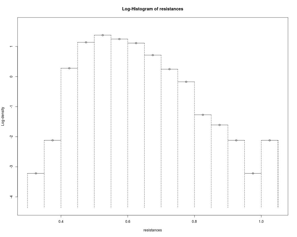
> logHist(resistances)
> ## Fit the hyperbolic distribution
> hyperbFit(resistances) 

Data:      resistances 
Parameter estimates:
     mu    delta    alpha     beta  
 0.3673   0.1369  67.2300  52.5829  
Likelihood:         426.7934 
criterion :         MLE 
Method:             Nelder-Mead 
Convergence code:   0 
Iterations:         423 
> 
> ## Actually fit.hyperb can deal with frequency data
> hyperbFit(resistors$midpoints, freq = resistors$counts)

Data:      resistors$midpoints 
Parameter estimates:
     mu    delta    alpha     beta  
 0.3673   0.1369  67.2300  52.5829  
Likelihood:         426.7934 
criterion :         MLE 
Method:             Nelder-Mead 
Convergence code:   0 
Iterations:         423 
> 
> 
> 
> 
> 
> 
> dev.off()
null device 
          1 
>