R Graphical Manual

Browse All

Last data update: 2014.03.03

R: Hill-Ekstrom calibration

HillEkstromCalib

R Documentation

Hill-Ekstrom calibration

Description

Hill-Ekstrom calibration for one or multiple stationary periods.

Usage

HillEkstromCalib(tFirst, tSecond, type, twl, site, start.angle = -6,
  distanceFilter = FALSE, distance, plot = TRUE)

Arguments

`tFirst`	vector of sunrise/sunset times (e.g. 2008-12-01 08:30).
`tSecond`	vector of of sunrise/sunset times (e.g. 2008-12-01 17:30).
`type`	vector of either 1 or 2, defining `tFirst` as sunrise or sunset respectively.
`twl`	data.frame containing twilights and at least `tFirst`, `tSecond` and `type` (alternatively give each parameter separately).
`site`	a `numerical vector` assigning each row to a particular period. Stationary periods in numerical order and values >0, migration/movement periods 0
`start.angle`	a single sun elevation angle. The combined process of checking for minimal variance in resulting latitude, which is the initial value for the sun elevation angle in the iterative process of identifying the latitudes with the least variance
`distanceFilter`	logical, if TRUE the `distanceFilter` will be used to filter unrealistic positions
`distance`	if `distanceFilter` is set `TRUE` a threshold distance in km has to be set (see: `distanceFilter`)
`plot`	logical, if TRUE the function will give a plot with all relevant information

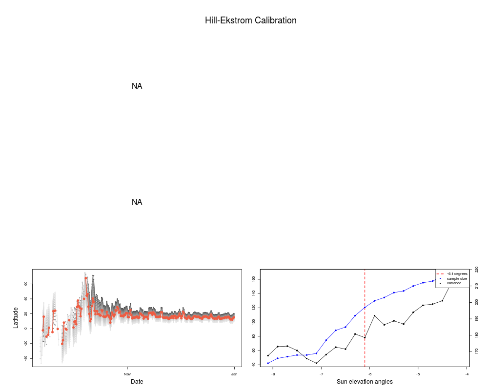
Details

The Hill-Ekstrom calibration has been suggested by Hill & Braun (2001) and Ekstrom (2004), and allows for calibrating data during stationary periods at unknown latitudinal positions. The Hill-Ekstrom calibration bases on an increasing error range in latitudes with an increasing mismatch between light level threshold and the used sun angle. This error is strongly amplified with proximity to the equinox times due to decreasing slope of day length variation with latitude. Furthermore, the sign of the error switches at the equinox, i.e. latitude is overestimated before the equinox and underestimated after the equinox (or vice versa depending on autumnal/vernal equinox, hemisphere, and sign of the mismatch between light level threshold and sun angle). When calculating the positions of a stationary period, the variance in latitude is minimal if the sun elevation angle fits to the defined light level threshold. Moreover, the accuracy of positions increases with decreasing variance in latitudes. However, the method is only applicable for stationary periods and under stable shading intensities. The plot produced by the function may help to judge visually if the calculated sun elevation angles are realistic (e.g. site 2 in the example below) or not (e.g. site 3 in the example below.

Value

A vector of sun elevation angles corresponding to the Hill-Ekstrom calibration for each defined period.

Author(s)

Simeon Lisovski

References

Ekstrom, P.A. (2004) An advance in geolocation by light. Memoirs of the National Institute of Polar Research, Special Issue, 58, 210-226.

Hill, C. & Braun, M.J. (2001) Geolocation by light level - the next step: Latitude. In: Electronic Tagging and Tracking in Marine Fisheries (eds J.R. Sibert & J. Nielsen), pp. 315-330. Kluwer Academic Publishers, The Netherlands.

Lisovski, S., Hewson, C.M, Klaassen, R.H.G., Korner-Nievergelt, F., Kristensen, M.W & Hahn, S. (2012) Geolocation by light: Accuracy and precision affected by environmental factors. Methods in Ecology and Evolution, DOI: 10.1111/j.2041-210X.2012.00185.x.

Examples

data(hoopoe2)
  hoopoe2$tFirst <- as.POSIXct(hoopoe2$tFirst, tz = "GMT")
  hoopoe2$tSecond <- as.POSIXct(hoopoe2$tSecond, tz = "GMT")
residency <- with(hoopoe2, changeLight(tFirst,tSecond,type, rise.prob=0.1,
                  set.prob=0.1, plot=FALSE, summary=FALSE))
HillEkstromCalib(hoopoe2,site = residency$site)

Results


R version 3.3.1 (2016-06-21) -- "Bug in Your Hair"
Copyright (C) 2016 The R Foundation for Statistical Computing
Platform: x86_64-pc-linux-gnu (64-bit)

R is free software and comes with ABSOLUTELY NO WARRANTY.
You are welcome to redistribute it under certain conditions.
Type 'license()' or 'licence()' for distribution details.

R is a collaborative project with many contributors.
Type 'contributors()' for more information and
'citation()' on how to cite R or R packages in publications.

Type 'demo()' for some demos, 'help()' for on-line help, or
'help.start()' for an HTML browser interface to help.
Type 'q()' to quit R.

> library(GeoLight)
Loading required package: maps

 # maps v3.1: updated 'world': all lakes moved to separate new #
 # 'lakes' database. Type '?world' or 'news(package="maps")'.  #


> png(filename="/home/ddbj/snapshot/RGM3/R_CC/result/GeoLight/HillEkstromCalib.Rd_%03d_medium.png", width=480, height=480)
> ### Name: HillEkstromCalib
> ### Title: Hill-Ekstrom calibration
> ### Aliases: HillEkstromCalib
> 
> ### ** Examples
> 
> data(hoopoe2)
>   hoopoe2$tFirst <- as.POSIXct(hoopoe2$tFirst, tz = "GMT")
>   hoopoe2$tSecond <- as.POSIXct(hoopoe2$tSecond, tz = "GMT")
> residency <- with(hoopoe2, changeLight(tFirst,tSecond,type, rise.prob=0.1,
+                   set.prob=0.1, plot=FALSE, summary=FALSE))
> HillEkstromCalib(hoopoe2,site = residency$site)
[1]   NA   NA -6.1
> 
> 
> 
> 
> 
> dev.off()
null device 
          1 
>