R Graphical Manual

Browse All

Last data update: 2014.03.03

R: Exact sampler for Gibbs Random Fields

exact.mrf

R Documentation

Exact sampler for Gibbs Random Fields

Description

exact.mrf gives exact sample from the likelihood of a general Potts model defined on a rectangular h x w lattice (h ≤ w) with either a first order or a second order dependency structure and a small number of rows (up to 19 for 2-state models).

Usage

exact.mrf(h, w, param, ncolors = 2, nei = 4,  
          pot = NULL, top = NULL, left = NULL, 
          bottom = NULL, right = NULL, corner = NULL, view = FALSE)

Arguments

`h`	the number of rows of the rectangular lattice.
`w`	the number of columns of the rectangular lattice.
`param`	numeric entry setting the interaction parameter (edges parameter)
`ncolors`	the number of states for the discrete random variables. By default, ncolors = 2.
`nei`	the number of neighbors. The latter must be one of nei = 4 or nei = 8, which respectively correspond to a first order and a second order dependency structure. By default, nei = 4.
`pot`	numeric entry setting homogeneous potential on singletons (vertices parameter). By default, pot = NULL
`top, left, bottom, right, corner`	numeric entry setting constant borders for the lattice. By default, top = NULL, left = NULL, bottom = NULL, right = NULL, corner = NULL.
`view`	Logical value indicating whether the draw should be printed. Do not display the optional borders.

References

Friel, N. and Rue, H. (2007). Recursive computing and simulation-free inference for general factorizable models. Biometrika, 94(3):661–672.

Examples

# Dimension of the lattice
height <- 8
width <- 10

# Interaction parameter
Beta <- 0.6 # Isotropic configuration
# Beta <- c(0.6, 0.6) # Anisotropic configuration when nei = 4
# Beta <- c(0.6, 0.6, 0.6, 0.6) # Anisotropic configuration when nei = 8

# Number of colors
K <- 2 
# Number of neighbors 
G <- 4

# Optional potential on sites
potential <- runif(K,-1,1)
# Optional borders. 
Top <- Bottom <- sample(0:(K-1), width, replace = TRUE)
Left <- Right <- sample(0:(K-1), height, replace = TRUE)
Corner <- sample(0:(K-1), 4, replace = TRUE)

# Exact sampling for the default setting
exact.mrf(h = height, w = width, param = Beta, view = TRUE)

# When specifying the number of colors and neighbors
exact.mrf(h = height, w = width, ncolors = K, nei = G, param = Beta, 
          view = TRUE)
          
# When specifying an optional potential on sites
exact.mrf(h = height, w = width, ncolors = K, nei = G, param = Beta, 
       pot = potential, view = TRUE)
       
# When specifying possible borders. The users will omit to mention all
# the non-existing borders
exact.mrf(h = height, w = width, ncolors = K, nei = G, param = Beta, 
       top = Top, left = Left, bottom = Bottom, right = Right, corner = Corner, view = TRUE)

Results


R version 3.3.1 (2016-06-21) -- "Bug in Your Hair"
Copyright (C) 2016 The R Foundation for Statistical Computing
Platform: x86_64-pc-linux-gnu (64-bit)

R is free software and comes with ABSOLUTELY NO WARRANTY.
You are welcome to redistribute it under certain conditions.
Type 'license()' or 'licence()' for distribution details.

R is a collaborative project with many contributors.
Type 'contributors()' for more information and
'citation()' on how to cite R or R packages in publications.

Type 'demo()' for some demos, 'help()' for on-line help, or
'help.start()' for an HTML browser interface to help.
Type 'q()' to quit R.

> library(GiRaF)
> png(filename="/home/ddbj/snapshot/RGM3/R_CC/result/GiRaF/exact.mrf.Rd_%03d_medium.png", width=480, height=480)
> ### Name: exact.mrf
> ### Title: Exact sampler for Gibbs Random Fields
> ### Aliases: exact.mrf
> 
> ### ** Examples
> 
> # Dimension of the lattice
> height <- 8
> width <- 10
> 
> # Interaction parameter
> Beta <- 0.6 # Isotropic configuration
> # Beta <- c(0.6, 0.6) # Anisotropic configuration when nei = 4
> # Beta <- c(0.6, 0.6, 0.6, 0.6) # Anisotropic configuration when nei = 8
> 
> # Number of colors
> K <- 2 
> # Number of neighbors 
> G <- 4
> 
> # Optional potential on sites
> potential <- runif(K,-1,1)
> # Optional borders. 
> Top <- Bottom <- sample(0:(K-1), width, replace = TRUE)
> Left <- Right <- sample(0:(K-1), height, replace = TRUE)
> Corner <- sample(0:(K-1), 4, replace = TRUE)
> 
> # Exact sampling for the default setting
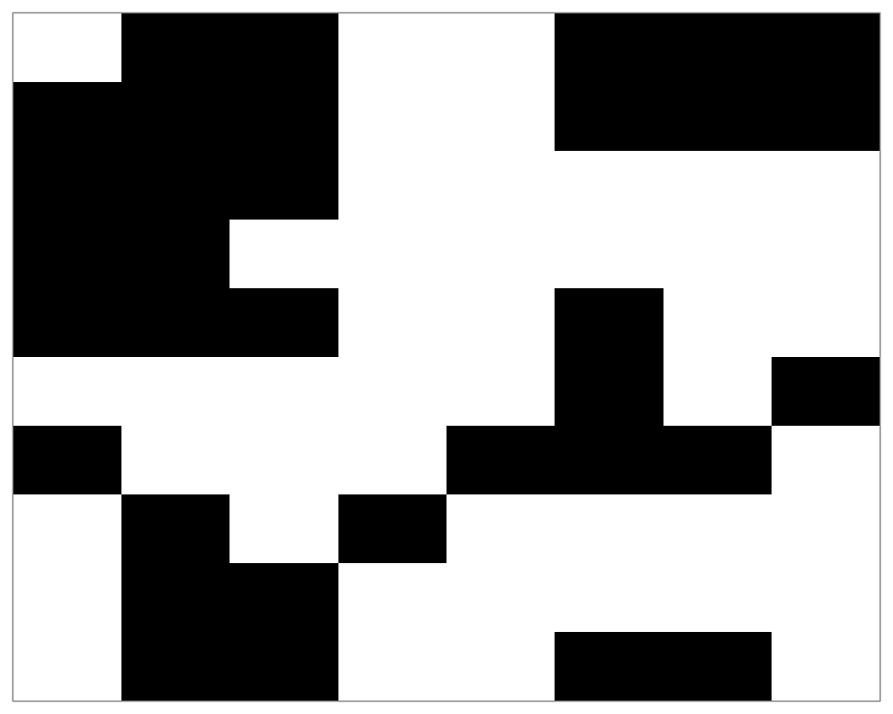
> exact.mrf(h = height, w = width, param = Beta, view = TRUE)
     [,1] [,2] [,3] [,4] [,5] [,6] [,7] [,8] [,9] [,10]
[1,]    1    1    0    1    1    1    1    1    1     1
[2,]    1    1    1    0    1    1    1    1    1     1
[3,]    1    1    0    1    1    1    1    0    0     0
[4,]    1    1    0    1    1    1    1    1    0     1
[5,]    1    0    1    1    0    1    1    1    1     0
[6,]    1    0    1    0    0    0    0    1    1     0
[7,]    1    0    0    0    0    1    0    1    1     0
[8,]    1    1    0    0    1    1    1    1    1     1
> 
> # When specifying the number of colors and neighbors
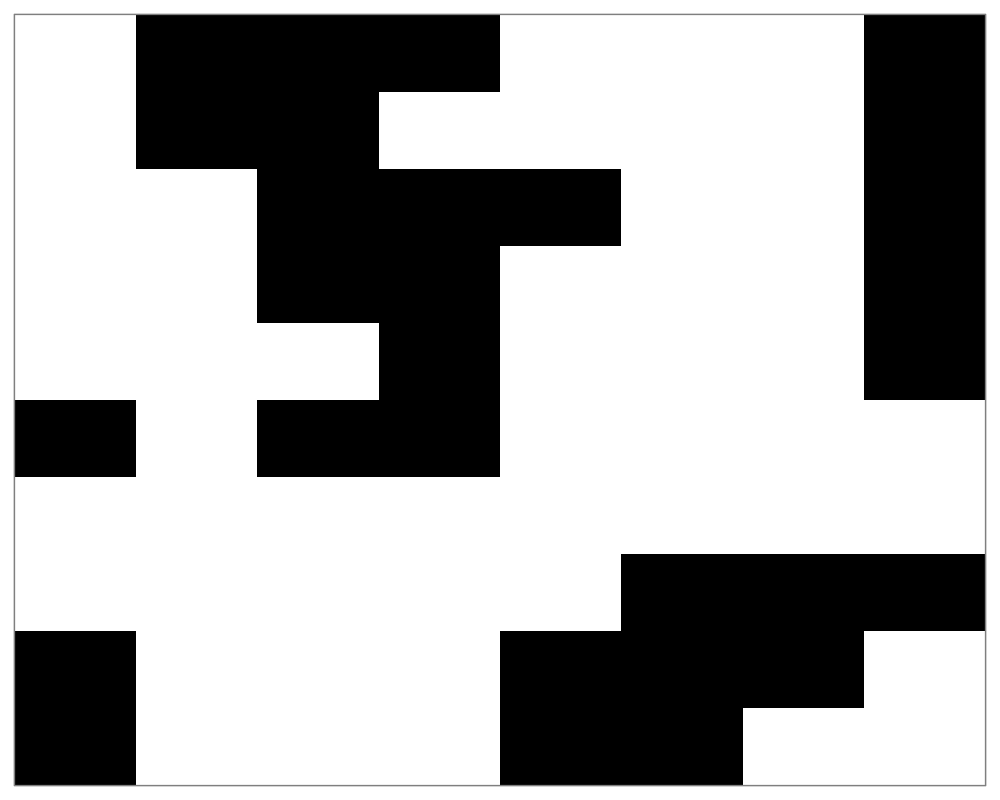
> exact.mrf(h = height, w = width, ncolors = K, nei = G, param = Beta, 
+           view = TRUE)
     [,1] [,2] [,3] [,4] [,5] [,6] [,7] [,8] [,9] [,10]
[1,]    1    1    1    1    1    0    1    1    1     0
[2,]    1    1    1    1    1    0    1    1    1     0
[3,]    1    0    1    1    1    1    1    1    1     1
[4,]    0    1    1    1    1    1    1    1    1     0
[5,]    0    0    1    1    1    0    0    1    0     0
[6,]    0    0    1    1    1    1    0    0    0     0
[7,]    1    0    0    0    1    1    0    0    0     1
[8,]    0    0    0    1    1    0    1    1    1     0
>           
> # When specifying an optional potential on sites
> exact.mrf(h = height, w = width, ncolors = K, nei = G, param = Beta, 
+        pot = potential, view = TRUE)
     [,1] [,2] [,3] [,4] [,5] [,6] [,7] [,8] [,9] [,10]
[1,]    1    1    1    1    1    1    1    1    1     1
[2,]    1    1    1    1    1    1    1    1    1     1
[3,]    1    1    1    1    1    1    1    0    0     1
[4,]    1    1    1    1    1    1    1    1    1     1
[5,]    1    1    1    1    1    1    0    1    1     1
[6,]    1    1    1    1    1    1    1    1    1     1
[7,]    1    1    1    1    1    1    1    1    1     1
[8,]    1    1    1    1    1    1    1    1    1     1
>        
> # When specifying possible borders. The users will omit to mention all
> # the non-existing borders
> exact.mrf(h = height, w = width, ncolors = K, nei = G, param = Beta, 
+        top = Top, left = Left, bottom = Bottom, right = Right, corner = Corner, view = TRUE)
     [,1] [,2] [,3] [,4] [,5] [,6] [,7] [,8] [,9] [,10]
[1,]    1    1    0    0    0    1    1    0    0     0
[2,]    1    1    1    0    0    1    0    0    0     0
[3,]    0    1    0    0    0    1    0    0    0     0
[4,]    1    0    0    0    0    0    0    0    0     1
[5,]    0    0    0    0    0    0    0    0    0     0
[6,]    1    0    1    1    0    0    1    1    1     0
[7,]    0    0    1    1    1    0    0    1    1     1
[8,]    1    1    0    1    1    0    0    0    1     1
> 
> 
> 
> 
> 
> dev.off()
null device 
          1 
>