Supported by Dr. Osamu Ogasawara and  . . |
|
Last data update: 2014.03.03 |
Plot a spline in a Cox regression modelDescriptionThis function is a more specialized version of the UsageplotHR(models, term = 1, se = TRUE, cntrst = ifelse(inherits(models, "rms") || inherits(models[[1]], "rms"), TRUE, FALSE), polygon_ci = TRUE, rug = "density", xlab = "", ylab = "Hazard Ratio", main = NULL, xlim = NULL, ylim = NULL, col.term = "#08519C", col.se = "#DEEBF7", col.dens = grey(0.9), lwd.term = 3, lty.term = 1, lwd.se = lwd.term, lty.se = lty.term, x.ticks = NULL, y.ticks = NULL, ylog = TRUE, cex = 1, y_axis_side = 2, plot.bty = "n", axes = TRUE, alpha = 0.05, ...) Arguments
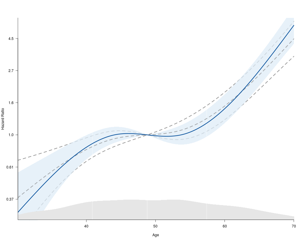
ValueThe function does not return anything Multiple models in one plotThe function allows for plotting multiple splines in one graph. Sometimes you might want to show more than one spline for the same variable. This allows you to create that comparison. Examples of a situation where I've used multiple splines in one plot is when I want to look at a variables behavior in different time periods. This is another way of looking at the proportional hazards assumption. The Schoenfeld residuals can be a little tricky to look at when you have the splines. Another example of when I've used this is when I've wanted to plot adjusted and unadjusted splines. This can very nicely demonstrate which of the variable span is mostly confounded. For instance - younger persons may exhibit a higher risk for a procedure but when you put in your covariates you find that the increased hazard changes back to the basic Author(s)Reinhard Seifert, Max Gordon Examples
library(survival)
library(rms)
# Get data for example
n <- 1000
set.seed(731)
age <- round(50 + 12*rnorm(n), 1)
label(age) <- "Age"
sex <- factor(sample(c('Male','Female'), n,
rep=TRUE, prob=c(.6, .4)))
cens <- 15*runif(n)
smoking <- factor(sample(c('Yes','No'), n,
rep=TRUE, prob=c(.2, .75)))
h <- .02*exp(.02*(age-50)+.1*((age-50)/10)^3+.8*(sex=='Female')+2*(smoking=='Yes'))
dt <- -log(runif(n))/h
label(dt) <- 'Follow-up Time'
e <- ifelse(dt <= cens,1,0)
dt <- pmin(dt, cens)
units(dt) <- "Year"
# Add missing data to smoking
smoking[sample(1:n, round(n*0.05))] <- NA
# Create a data frame since plotHR will otherwise
# have a hard time getting the names of the variables
ds <- data.frame(
dt = dt,
e = e,
age=age,
smoking=smoking,
sex=sex)
library(splines)
Srv <- Surv(dt,e)
fit.coxph <- coxph(Srv ~ bs(age, 3) + sex + smoking, data=ds)
org_par <- par(xaxs="i", ask=TRUE)
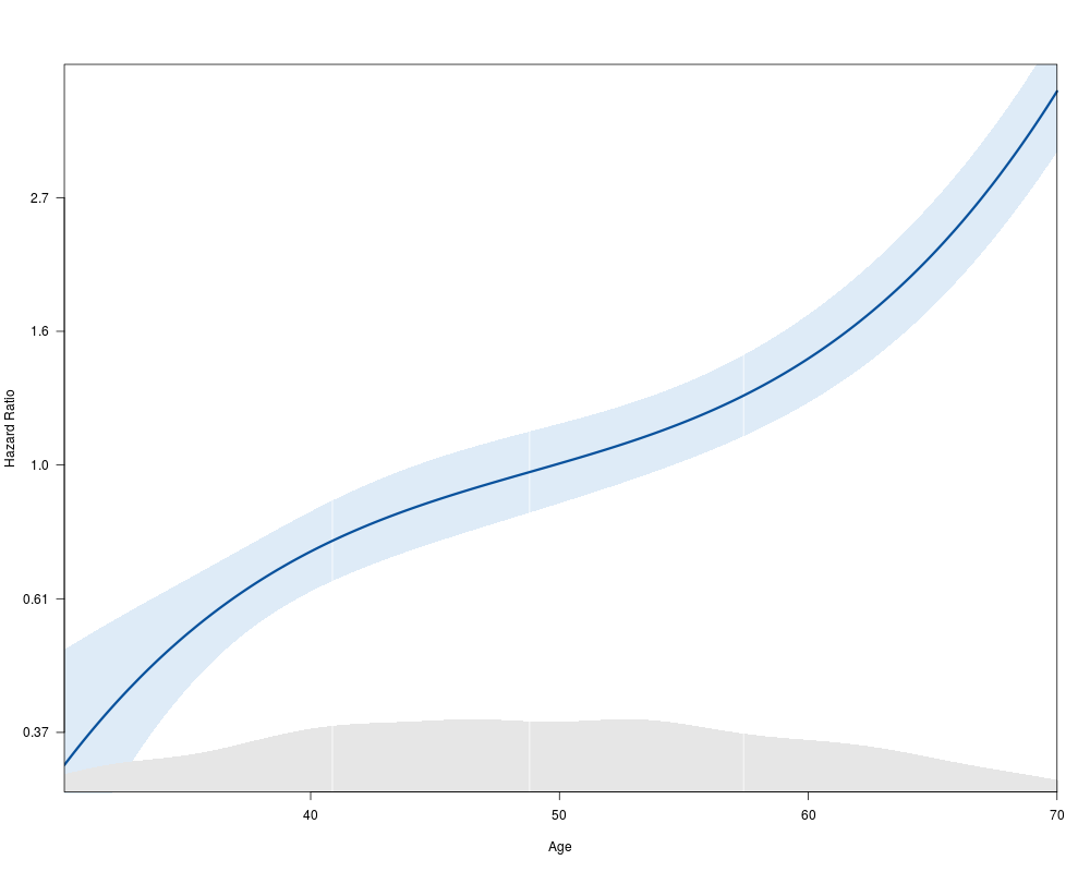
plotHR(fit.coxph, term="age", plot.bty="o", xlim=c(30, 70), xlab="Age")
dd <- datadist(ds)
options(datadist='dd')
fit.cph <- cph(Srv ~ rcs(age,4) + sex + smoking, data=ds, x=TRUE, y=TRUE)
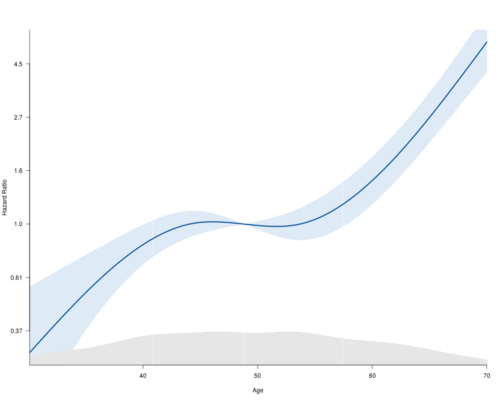
plotHR(fit.cph, term=1, plot.bty="l", xlim=c(30, 70), xlab="Age")
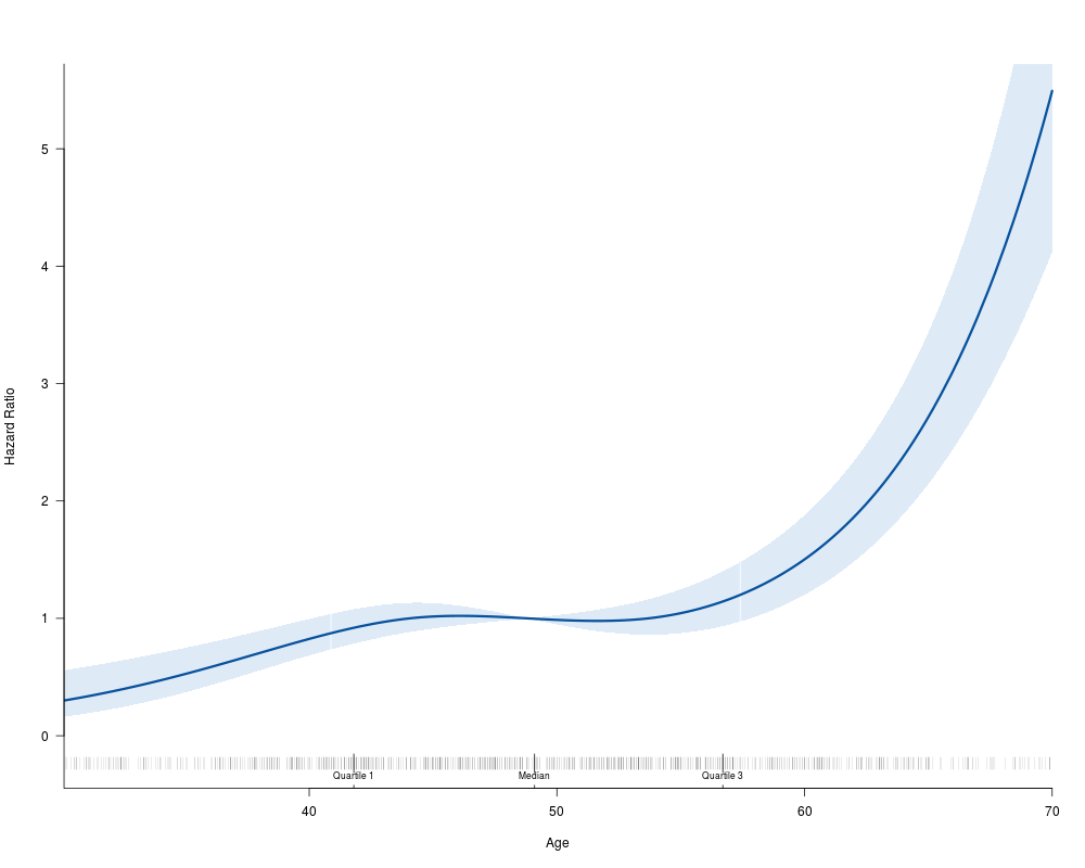
plotHR(fit.cph, term="age", plot.bty="l", xlim=c(30, 70), ylog=FALSE, rug="ticks", xlab="Age")
unadjusted_fit <- cph(Srv ~ rcs(age,4), data=ds, x=TRUE, y=TRUE)
plotHR(list(fit.cph, unadjusted_fit), term="age", xlab="Age",
polygon_ci=c(TRUE, FALSE),
col.term = c("#08519C", "#77777799"),
col.se = c("#DEEBF7BB", grey(0.6)),
lty.term = c(1, 2),
plot.bty="l", xlim=c(30, 70))
par(org_par)
Results
R version 3.3.1 (2016-06-21) -- "Bug in Your Hair"
Copyright (C) 2016 The R Foundation for Statistical Computing
Platform: x86_64-pc-linux-gnu (64-bit)

R is free software and comes with ABSOLUTELY NO WARRANTY.
You are welcome to redistribute it under certain conditions.
Type 'license()' or 'licence()' for distribution details.

R is a collaborative project with many contributors.
Type 'contributors()' for more information and
'citation()' on how to cite R or R packages in publications.

Type 'demo()' for some demos, 'help()' for on-line help, or
'help.start()' for an HTML browser interface to help.
Type 'q()' to quit R.

> library(Greg)
Loading required package: forestplot
Loading required package: grid
Loading required package: magrittr
Loading required package: Gmisc
Loading required package: Rcpp
Loading required package: htmlTable
> png(filename="/home/ddbj/snapshot/RGM3/R_CC/result/Greg/plotHR.Rd_%03d_medium.png", width=480, height=480)
> ### Name: plotHR
> ### Title: Plot a spline in a Cox regression model
> ### Aliases: plotHR
>
> ### ** Examples
>
> library(survival)
> library(rms)
Loading required package: Hmisc
Loading required package: lattice
Loading required package: Formula
Loading required package: ggplot2

Attaching package: 'Hmisc'

The following objects are masked from 'package:base':

    format.pval, round.POSIXt, trunc.POSIXt, units

Loading required package: SparseM

Attaching package: 'SparseM'

The following object is masked from 'package:base':

    backsolve

>
> # Get data for example
> n <- 1000
> set.seed(731)
>
> age <- round(50 + 12*rnorm(n), 1)
> label(age) <- "Age"
>
> sex <- factor(sample(c('Male','Female'), n,
+     rep=TRUE, prob=c(.6, .4)))
> cens <- 15*runif(n)
>
> smoking <- factor(sample(c('Yes','No'), n,
+     rep=TRUE, prob=c(.2, .75)))
>
> h <- .02*exp(.02*(age-50)+.1*((age-50)/10)^3+.8*(sex=='Female')+2*(smoking=='Yes'))
> dt <- -log(runif(n))/h
> label(dt) <- 'Follow-up Time'
>
> e <- ifelse(dt <= cens,1,0)
> dt <- pmin(dt, cens)
> units(dt) <- "Year"
>
> # Add missing data to smoking
> smoking[sample(1:n, round(n*0.05))] <- NA
>
> # Create a data frame since plotHR will otherwise
> # have a hard time getting the names of the variables
> ds <- data.frame(
+   dt = dt,
+   e = e,
+   age=age,
+   smoking=smoking,
+   sex=sex)
>
> library(splines)
> Srv <- Surv(dt,e)
> fit.coxph <- coxph(Srv ~ bs(age, 3) + sex + smoking, data=ds)
>
> org_par <- par(xaxs="i", ask=TRUE)
> plotHR(fit.coxph, term="age", plot.bty="o", xlim=c(30, 70), xlab="Age")
>
> dd <- datadist(ds)
> options(datadist='dd')
> fit.cph <- cph(Srv ~ rcs(age,4) + sex + smoking, data=ds, x=TRUE, y=TRUE)
>
> plotHR(fit.cph, term=1, plot.bty="l", xlim=c(30, 70), xlab="Age")
>
> plotHR(fit.cph, term="age", plot.bty="l", xlim=c(30, 70), ylog=FALSE, rug="ticks", xlab="Age")
>
> unadjusted_fit <- cph(Srv ~ rcs(age,4), data=ds, x=TRUE, y=TRUE)
> plotHR(list(fit.cph, unadjusted_fit), term="age", xlab="Age",
+ 		polygon_ci=c(TRUE, FALSE),
+ 		col.term = c("#08519C", "#77777799"),
+ 		col.se = c("#DEEBF7BB", grey(0.6)),
+ 		lty.term = c(1, 2),
+ 		plot.bty="l", xlim=c(30, 70))
> par(org_par)
>
>
>
>
>
> dev.off()
null device
          1
>
|