R Graphical Manual

Browse All

Last data update: 2014.03.03

R: Constructing confidence intervals for the Generalized...

gsym.point

R Documentation

Constructing confidence intervals for the Generalized Symmetry point and its accuracy measures through two methods

Description

gsym.point constructs confidence intervals for the Generalized Symmetry point and its accuracy measures sensitivity and specificity for a continuous diagnostic test using two methods: the Generalized Pivotal Quantity method and the Empirical Likelihood method.

Usage

gsym.point (methods, data, marker, status, tag.healthy, categorical.cov = NULL, 
CFN = 1, CFP = 1, control = control.gsym.point(), confidence.level = 0.95, 
trace = FALSE, seed = FALSE, value.seed = 3)

Arguments

`methods`	a character vector selecting the method(s) to be used for estimating the Generalized Symmetry point and its accuracy measures. The possible options are: "GPQ", "EL", or both: c("GPQ","EL") or c("EL","GPQ").
`data`	a data frame containing all needed variables: the diagnostic marker, the true disease status and when it is neccesary, the categorical covariate.
`marker`	a character string with the name of the diagnostic test variable.
`status`	a character string with the name of the variable that distinguishes healthy from diseased individuals.
`tag.healthy`	the value codifying healthy individuals in the `status` variable.
`categorical.cov`	a character string with the name of the categorical covariate according to which the Generalized Symmetry point (optimal cutpoint) is to be calculated. The default is NULL (no categorical covariate is considered in the analysis).
`CFN`	a numerical value. It specifies the cost of a false negative decision. The default value is 1.
`CFP`	a numerical value. It specifies the cost of a false positive decision. The default value is 1.
`control`	output of the `control.gsym.point` function, which controls the whole optimal-cutpoint calculation process.
`confidence.level`	a numerical value with the confidence level for the construction of the confidence intervals. The default value is 0.95.
`trace`	a logical value. If TRUE, information on progress is shown. The default is FALSE.
`seed`	a logical value. If TRUE, a seed is fixed for generating the trials in the computation of the confidence intervals. The default is FALSE.
`value.seed`	If `seed` is TRUE, it is the numerical value for the fixed seed. The default value is 3.

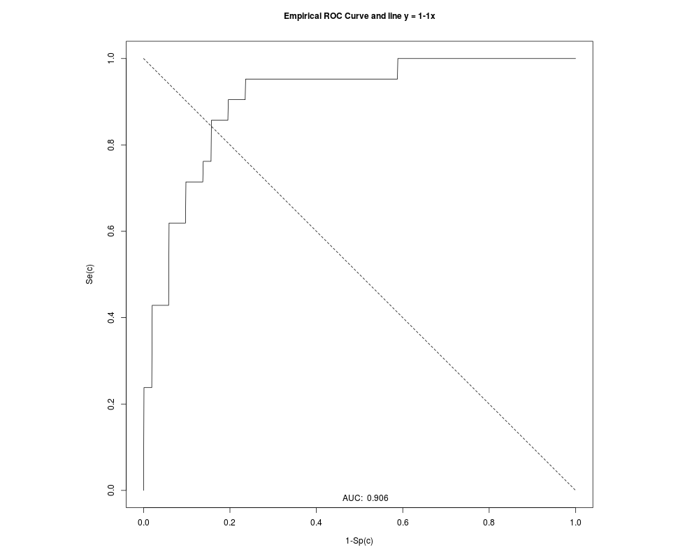
Details

The Symmetry point c_{S} satisfies the equality p(c_{S}) = q(c_{S}), where p and q denote, respectively, the specificity (or true negative fraction) and sensitivity (or true positive fraction). Geometrically, it is the point where the ROC curve and the line y = 1 - x (the perpendicular to the positive diagonal line) intersect, and it can also be seen as the point that maximizes simultaneously both types of correct classifications (Riddle and Stratford, 1999; Gallop et al., 2003) corresponding, therefore, to the probability of correctly classifying any subject, whether it is healthy or diseased (Jim<c3><a9>nez-Valverde et al., 2012; 2014).

Taking into account the costs associated to the false positives and false negatives misclassifications C_{FP} and C_{FN}, an extension of the Symmetry point, the Generalized Symmetry point c_{GS}, can be defined as follows (L<c3><b3>pez-Rat<c3><b3>n et al., 2015):

ρ (1-p(c_{GS})) = 1-q(c_{GS})

where ρ = frac{C_{FP}}{C_{FN}} is the relative loss (cost) of a false positive classification as compared with a false negative classification. Analogously to the Symmetry point, c_{GS} is obtained graphically by the intersection point between the ROC curve and the line y = 1 - ρ x.

In this package, the two methods proposed in L<c3><b3>pez-Rat<c3><b3>n et al. (2015) for estimating the Generalized Symmetry point and its sensitivity and specificity indexes are available:

"GPQ": Method based on the Generalized Pivotal Quantity (Weerahandi, 1993; 1995; Lai et al., 2012). It assumes that the diagnostic test on both groups or a monotone Box-Cox transformation is Normal distributed. So, the Generalized Symmetry point c_{GS} can be estimated from the following equation:

Φ(a+bΦ^{-1}(t)) = 1-ρ t Leftrightarrow Φ ≤ft(frac{Φ^{-1}(1-ρ t)-a}{b} ight)-t=0

where a=frac{μ_1-μ_0}{σ_1}, b=frac{σ_0}{σ_1}, t=1-p(c_{GS}) and Φ denotes the standard Normal cumulative distribution function (cdf), with μ_i and σ_i, i = 0,1, the mean and standard deviation of healthy (i=0) and diseased (i=1) populations, respectively. To check the assumption of normality, the Shapiro-Wilk test is used with a significance level of 5%.

"EL": Method based on the Empirical Likelihood (Thomas and Grunkemeier, 1975). It takes into account that c_{GS} can be seen as two specific quantiles, the p(c_{GS})-th quantile of the healthy population and the ρ (1-q(c_{GS}))-th quantile of the diseased population. Following the same reasoning as in Molanes-L<c3><b3>pez and Let<c3><b3>n (2011), and considering that the value of p(c_{GS}) is known in advance and the Generalized Symmetry point defines an operating point on the ROC curve fulfilling 1-x=p(c_{GS}), the following adjusted empirical log-likelihood ratio function is derived to make inference on c_{GS}:

ell(c)=2n_0hat{F}_{0,g_{0}}(c)log!≤ft(frac{hat{F}_{0,g_{0}}(c)}{p(c)} ight) +2n_0(1-hat{F}_{0,g_{0}}(c))log≤ft(frac{1-hat{F}_{0,g_0}(c)}{1-p(c)} ight)

+2n_1hat{F}_{1,g_{1}}(c)log≤ft(frac{hat{F}_{1,g_{1}}(c)}{ρ(1-p(c))} ight) +2n_1(1-hat{F}_{1,g_{1}}(c))log≤ft(frac{1-hat{F}_{1,g_{1}}(c)}{1-ρ (1-p(c))} ight)!,

where hat{F}_{i,g_{i}}(y)=frac{1}{n_i}∑_{k_i=1}^{n_i}K≤ft(frac{y-Y_{ik_i}}{g_{i}} ight) are kernel-type estimates of the cdfs F_{i}, of the two populations, i=0,1, with K(y)=int_{-∞}^{y} K(z)mathrm{d}z a kernel function and g_i the smoothing parameter, for i=0,1.

Value

Returns an object of class "gsym.point" with the following components:

`methods`	a character vector with the value of the `methods` argument used in the call.
`levels.cat`	a character vector indicating the levels of the categorical covariate if the `categorical.cov` argument in the `gsym.point` function is not NULL.
`call`	the matched call.
`data`	the data frame with the variables used in the call.

For each of the methods used in the call, a list with the following components is obtained:

`"optimal.result"`	a list with the Generalized Symmetry point and its associated sensitivity and specificity accuracy measures with the corresponding confidence intervals.
`"AUC"`	a list with the numerical value of the Area Under the ROC Curve.
`"rho"`	the numerical value of the cost ratio ρ = frac{C_{FP}}{C_{FN}}.
`"pvalue.healthy"`	the numerical value of the p-value obtained by the Shapiro-Wilk normality test for checking the normality assumption of the marker in healthy population.
`"pvalue.diseased"`	the numerical value of the p-value obtained by the Shapiro-Wilk normality test for checking the normality assumption of the marker in diseased population.

In addition, if original data are not normally distributed the following components also appears:

`"lambda"`	the estimated numerical value of the power in the Box-Cox transformation.
`"normality.transformed"`	a character string indicating if the transformed marker values by the Box-Cox transformation are normally distributed ("yes") or not ("no").
`"pvalue.healthy.transformed"`	the numerical value of the p-value obtained by the Shapiro-Wilk normality test for checking the normality assumption of the Box-Cox transformed marker in healthy population.
`"pvalue.diseased.transformed"`	the numerical value of the p-value obtained by the Shapiro-Wilk normality test for checking the normality assumption of the Box-Cox transformed marker in diseased population.

Author(s)

M<c3><b3>nica L<c3><b3>pez-Rat<c3><b3>n, Carmen Cadarso-Su<c3><a1>rez, Elisa M. Molanes-L<c3><b3>pez and Emilio Let<c3><b3>n

References

Gallop, R.J., Crits-Christoph, P., Muenz, L.R. and Tu, X.M. (2003). Determination and interpretation of the optimal operating point for ROC curves derived through generalized linear models. Understanding Statistics 2, 219-242.

Jim<c3><a9>nez-Valverde, A. (2012). Insights into the area under the receiver operating characteristic curve (AUC) as a discrimination measure in species distribution modelling. Global Ecology and Biogeography 21, 498-507.

Jim<c3><a9>nez-Valverde, A. (2014). Threshold-dependence as a desirable attribute for discrimination assessment: implications for the evaluation of species distribution models. Biodiversity Conservation 23, 369-385

Lai, C.Y., Tian, L. and Schisterman, E.F. (2012). Exact confidence interval estimation for the Youden index and its corresponding optimal cut-point. Comput. Stat. Data Anal. 56, 1103-1114.

L<c3><b3>pez-Rat<c3><b3>n, M., Cadarso-Su<c3><a1>rez, C., Molanes-L<c3><b3>pez, E.M. and Let<c3><b3>n, E. (2015). Confidence intervals for the Symmetry point: an optimal cutpoint in continuous diagnostic tests. (Submitted).

Metz, C.E. (1978). Basic Principles of ROC Analysis. Seminars in Nuclear Medicine 8, 183-298.

Molanes-L<c3><b3>pez, E.M. and Let<c3><b3>n, E. (2011). Inference of the Youden index and associated threshold using empirical likelihood for quantiles. Statistics in Medicine 30, 2467-2480.

Molanes-L<c3><b3>pez, E.M., Van Keilegom, I. and Veraverbeke, N. (2009). Empirical likelihood for non-smooth criterion functions. Scandinavian Journal of Statistics 36, 413-432.

Remaley, A.T., Sampson, M.L., DeLeo, J.M., Remaley, N.A., Farsi, B.D. and Zweig, M.H. (1999). Prevalence-value-accuracy plots: a new method for comparing diagnostic tests based on misclassification costs. Clinical Chemistry 45, 934-941.

Riddle, D.L. and Stratford, P.W. (1999). Interpreting validity indexes for diagnostic tests: An illustration using the Berg Balance Test. Physical Therapy 79, 939-948.

Rutter, C.M. and Miglioretti, D.L. (2003). Estimating the accuracy of psychological scales using longitudinal data. Biostatistics 4, 97-107.

Thomas, D.R. and Grunkemeier, G.L. (1975). Confidence interval estimation of survival probabilities for censored data. Journal of the American Statistical Association 70, 865-871.

Wand, M.P. and Jones, M.C. (1995). Kernel smoothing. Chapman & Hall, London.

Weerahandi, S. (1993). Generalized confidence intervals. Journal of the American Statistical Association 88, 899-905.

Weerahandi, S. (1995). Exact statistical methods for data analysis. Springer-Verlag, New York.

Zhou, W. and Jing, B.Y. (2003). Adjusted empirical likelihood method for quantiles. Annals of the Institute of Statistical Mathematics 55, 689-703.

Examples

library(GsymPoint)

data(melanoma)

###########################################################
# marker: X
# status: group
###########################################################

###########################################################
# Generalized Pivotal Quantity Method ("GPQ"): 
# Original data normally distributed
###########################################################

gsym.point.GPQ.melanoma<-gsym.point(methods = "GPQ", data = melanoma,
marker = "X", status = "group", tag.healthy = 0, categorical.cov = NULL, 
CFN = 1, CFP = 1, control = control.gsym.point(),confidence.level = 0.95, 
trace = FALSE, seed = FALSE, value.seed = 3)

summary(gsym.point.GPQ.melanoma)

plot(gsym.point.GPQ.melanoma)


data(prostate)

###########################################################
# marker: marker
# status: status
###########################################################

###########################################################
# Generalized Pivotal Quantity Method ("GPQ"): 
# Box-Cox transformed data normally distributed
###########################################################

gsym.point.GPQ.prostate <- gsym.point (methods = "GPQ", data = prostate,
marker = "marker", status = "status", tag.healthy = 0, categorical.cov = NULL, 
CFN = 1, CFP = 1, control = control.gsym.point(), confidence.level = 0.95, 
trace = FALSE, seed = FALSE, value.seed = 3)

summary(gsym.point.GPQ.prostate)

plot(gsym.point.GPQ.prostate)


data(elastase)

###########################################################
# marker: elas
# status: status
###########################################################

###########################################################
# Generalized Pivotal Quantity Method ("GPQ"):
# Original data not normally distributed 
# Box-Cox transformed data not normally distributed
###########################################################

gsym.point.GPQ.elastase <- gsym.point(methods = "GPQ", data = elastase, 
marker = "elas", status = "status", tag.healthy = 0, categorical.cov = NULL, 
CFN = 1, CFP = 1, control = control.gsym.point(), confidence.level = 0.95, 
trace = FALSE, seed = FALSE, value.seed = 3) 

summary(gsym.point.GPQ.elastase)

plot(gsym.point.GPQ.elastase)

Results


R version 3.3.1 (2016-06-21) -- "Bug in Your Hair"
Copyright (C) 2016 The R Foundation for Statistical Computing
Platform: x86_64-pc-linux-gnu (64-bit)

R is free software and comes with ABSOLUTELY NO WARRANTY.
You are welcome to redistribute it under certain conditions.
Type 'license()' or 'licence()' for distribution details.

R is a collaborative project with many contributors.
Type 'contributors()' for more information and
'citation()' on how to cite R or R packages in publications.

Type 'demo()' for some demos, 'help()' for on-line help, or
'help.start()' for an HTML browser interface to help.
Type 'q()' to quit R.

> library(GsymPoint)
Loading required package: truncnorm
Loading required package: Rsolnp
> png(filename="/home/ddbj/snapshot/RGM3/R_CC/result/GsymPoint/gsym.point.Rd_%03d_medium.png", width=480, height=480)
> ### Name: gsym.point
> ### Title: Constructing confidence intervals for the Generalized Symmetry
> ###   point and its accuracy measures through two methods
> ### Aliases: gsym.point
> 
> ### ** Examples
> 
> library(GsymPoint)
> 
> data(melanoma)
> 
> ###########################################################
> # marker: X
> # status: group
> ###########################################################
> 
> ###########################################################
> # Generalized Pivotal Quantity Method ("GPQ"): 
> # Original data normally distributed
> ###########################################################
> 
> gsym.point.GPQ.melanoma<-gsym.point(methods = "GPQ", data = melanoma,
+ marker = "X", status = "group", tag.healthy = 0, categorical.cov = NULL, 
+ CFN = 1, CFP = 1, control = control.gsym.point(),confidence.level = 0.95, 
+ trace = FALSE, seed = FALSE, value.seed = 3)
> 
> summary(gsym.point.GPQ.melanoma)

*************************************************
OPTIMAL CUTOFF: GENERALIZED SYMMETRY POINT
*************************************************

Call:
gsym.point(methods = "GPQ", data = melanoma, marker = "X", status = "group", 
    tag.healthy = 0, categorical.cov = NULL, CFN = 1, CFP = 1, 
    control = control.gsym.point(), confidence.level = 0.95, 
    trace = FALSE, seed = FALSE, value.seed = 3)

According to the Shapiro-Wilk normality test, the marker can be
considered normally distributed in both groups.

Shapiro-Wilk test p-values

                Group 0 Group 1
Original marker  0.4719  0.9084

Area under the ROC curve (AUC):  0.906 

METHOD: GPQ

              Estimate 95% CI lower limit 95% CI upper limit
cutoff      -0.8273306         -1.3643851         -0.3205409
Specificity  0.8181698          0.7321867          0.8859924
Sensitivity  0.8181698          0.7321867          0.8859924



> 
> plot(gsym.point.GPQ.melanoma)
> 
> 
> data(prostate)
> 
> ###########################################################
> # marker: marker
> # status: status
> ###########################################################
> 
> ###########################################################
> # Generalized Pivotal Quantity Method ("GPQ"): 
> # Box-Cox transformed data normally distributed
> ###########################################################
> 
> gsym.point.GPQ.prostate <- gsym.point (methods = "GPQ", data = prostate,
+ marker = "marker", status = "status", tag.healthy = 0, categorical.cov = NULL, 
+ CFN = 1, CFP = 1, control = control.gsym.point(), confidence.level = 0.95, 
+ trace = FALSE, seed = FALSE, value.seed = 3)
> 
> summary(gsym.point.GPQ.prostate)

*************************************************
OPTIMAL CUTOFF: GENERALIZED SYMMETRY POINT
*************************************************

Call:
gsym.point(methods = "GPQ", data = prostate, marker = "marker", 
    status = "status", tag.healthy = 0, categorical.cov = NULL, 
    CFN = 1, CFP = 1, control = control.gsym.point(), confidence.level = 0.95, 
    trace = FALSE, seed = FALSE, value.seed = 3)

According to the Shapiro-Wilk normality test, the marker can not
be considered normally distributed in both groups. 
However, after transforming the marker using the Box-Cox 
transformation estimate, the Shapiro-Wilk normality test 
indicates that the transformed marker can be considered 
normally distributed in both groups.

Box-Cox lambda estimate = -1.2494 

Shapiro-Wilk test p-values
                           Group 0 Group 1
Original marker             0.0000  0.0232
Box-Cox transformed marker  0.3641  0.2118

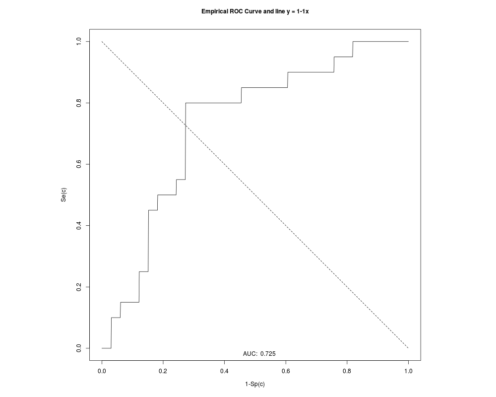
Area under the ROC curve (AUC):  0.725 

METHOD: GPQ

              Estimate 95% CI lower limit 95% CI upper limit
cutoff      64.6644705         59.9316210         70.3332623
Specificity  0.6589833          0.5496043          0.7621764
Sensitivity  0.6589833          0.5496043          0.7621764



> 
> plot(gsym.point.GPQ.prostate)
> 
> 
> data(elastase)
> 
> ###########################################################
> # marker: elas
> # status: status
> ###########################################################
> 
> ###########################################################
> # Generalized Pivotal Quantity Method ("GPQ"):
> # Original data not normally distributed 
> # Box-Cox transformed data not normally distributed
> ###########################################################
> 
> gsym.point.GPQ.elastase <- gsym.point(methods = "GPQ", data = elastase, 
+ marker = "elas", status = "status", tag.healthy = 0, categorical.cov = NULL, 
+ CFN = 1, CFP = 1, control = control.gsym.point(), confidence.level = 0.95, 
+ trace = FALSE, seed = FALSE, value.seed = 3) 
According to the Shapiro-Wilk normality test, the original marker 
can not be considered normally distributed in both groups.
After transforming the marker using the Box-Cox transformation 
estimate the Shapiro-Wilk normality test indicates that the 
transformed marker can not be considered normally distributed 
in both groups. 
Therefore, the results obtained with the GPQ method may not be 
reliable. You must use the EL method instead.

Box-Cox lambda estimate = 0.1136 

Shapiro-Wilk test p-values
                           Group 0 Group 1
Original marker             0.0746  0.0091
Box-Cox transformed marker  0.0000  0.0793
> 
> summary(gsym.point.GPQ.elastase)

*************************************************
OPTIMAL CUTOFF: GENERALIZED SYMMETRY POINT
*************************************************

Call:
gsym.point(methods = "GPQ", data = elastase, marker = "elas", 
    status = "status", tag.healthy = 0, categorical.cov = NULL, 
    CFN = 1, CFP = 1, control = control.gsym.point(), confidence.level = 0.95, 
    trace = FALSE, seed = FALSE, value.seed = 3)

According to the Shapiro-Wilk normality test, the original marker
can not be considered normally distributed in both groups.
After transforming the marker using the Box-Cox transformation
estimate the Shapiro-Wilk normality test indicates that the
transformed marker can not be considered normally distributed
in both groups.
Therefore, the results obtained with the GPQ method may not be
reliable. You must use the EL method instead.

Box-Cox lambda estimate = 0.1136 

Shapiro-Wilk test p-values
                           Group 0 Group 1
Original marker             0.0746  0.0091
Box-Cox transformed marker  0.0000  0.0793

Area under the ROC curve (AUC):  0.744 

METHOD: GPQ

              Estimate 95% CI lower limit 95% CI upper limit
cutoff      34.7162933         31.1720387         38.4310676
Specificity  0.6933122          0.6182304          0.7585386
Sensitivity  0.6933122          0.6182304          0.7585386



> 
> plot(gsym.point.GPQ.elastase)
> 
> 
> 
> 
> 
> 
> dev.off()
null device 
          1 
>