Default plotting of a gsym.point object

Description

On the basis of a gsym.point object, it plots the Receiver Operating Characteristic (ROC) curve and the line y = 1-ρ t.

Usage

## S3 method for class 'gsym.point'
plot(x, legend = TRUE, ...)

Arguments

Author(s)

M<c3><b3>nica L<c3><b3>pez-Rat<c3><b3>n, Carmen Cadarso-Su<c3><a1>rez, Elisa M. Molanes-L<c3><b3>pez and Emilio Let<c3><b3>n

See Also

gsym.point, control.gsym.point

Examples

library(GsymPoint)

data(melanoma)

###########################################################
# Generalized Pivotal Quantity Method ("GPQ"): 
###########################################################

gsym.point.GPQ.melanoma<-gsym.point(methods = "GPQ", data = melanoma,
marker = "X", status = "group", tag.healthy = 0, categorical.cov = NULL, 
CFN = 1, CFP = 1, control = control.gsym.point(),confidence.level = 0.95, 
trace = FALSE, seed = FALSE, value.seed = 3)

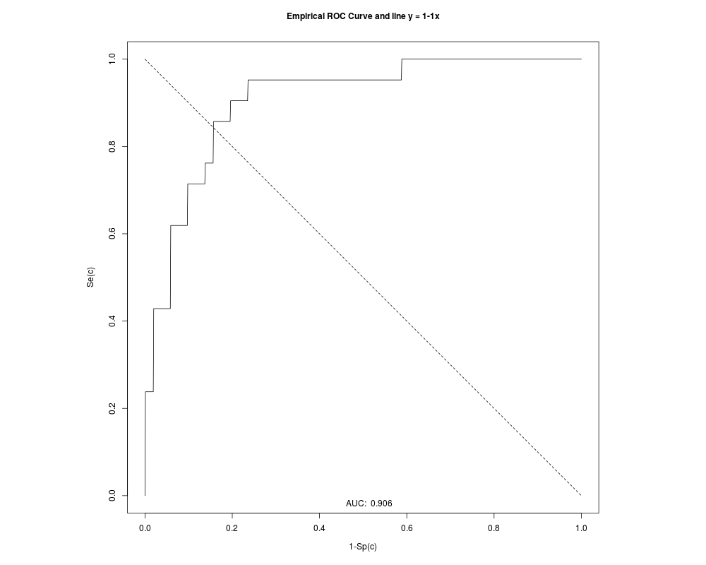
plot(gsym.point.GPQ.melanoma)


data(prostate)

###########################################################
# Generalized Pivotal Quantity Method ("GPQ"): 
###########################################################

gsym.point.GPQ.prostate <- gsym.point (methods = "GPQ", data = prostate,
marker = "marker", status = "status", tag.healthy = 0, categorical.cov = NULL, 
CFN = 1, CFP = 1, control = control.gsym.point(), confidence.level = 0.95, 
trace = FALSE, seed = FALSE, value.seed = 3)

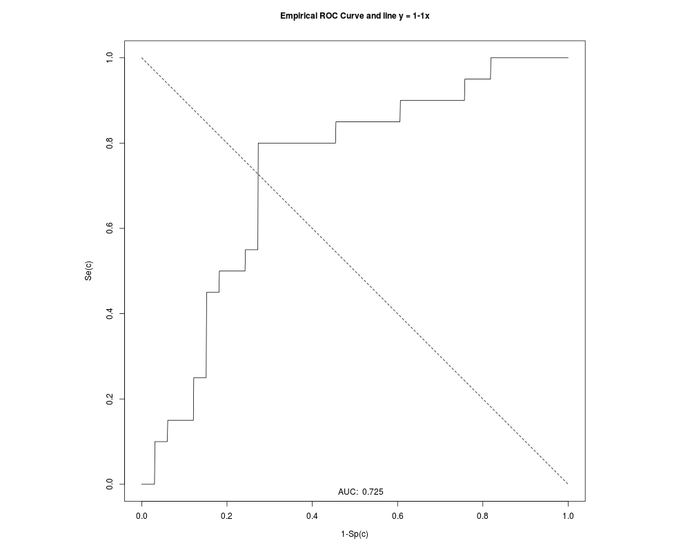
plot(gsym.point.GPQ.prostate)


data(elastase)

###########################################################
# Generalized Pivotal Quantity Method ("GPQ"): 
###########################################################

gsym.point.GPQ.elastase <- gsym.point(methods = "GPQ", data = elastase, 
marker = "elas", status = "status", tag.healthy = 0, categorical.cov = NULL, 
CFN = 1, CFP = 1, control = control.gsym.point(), confidence.level = 0.95, 
trace = FALSE, seed = FALSE, value.seed = 3) 

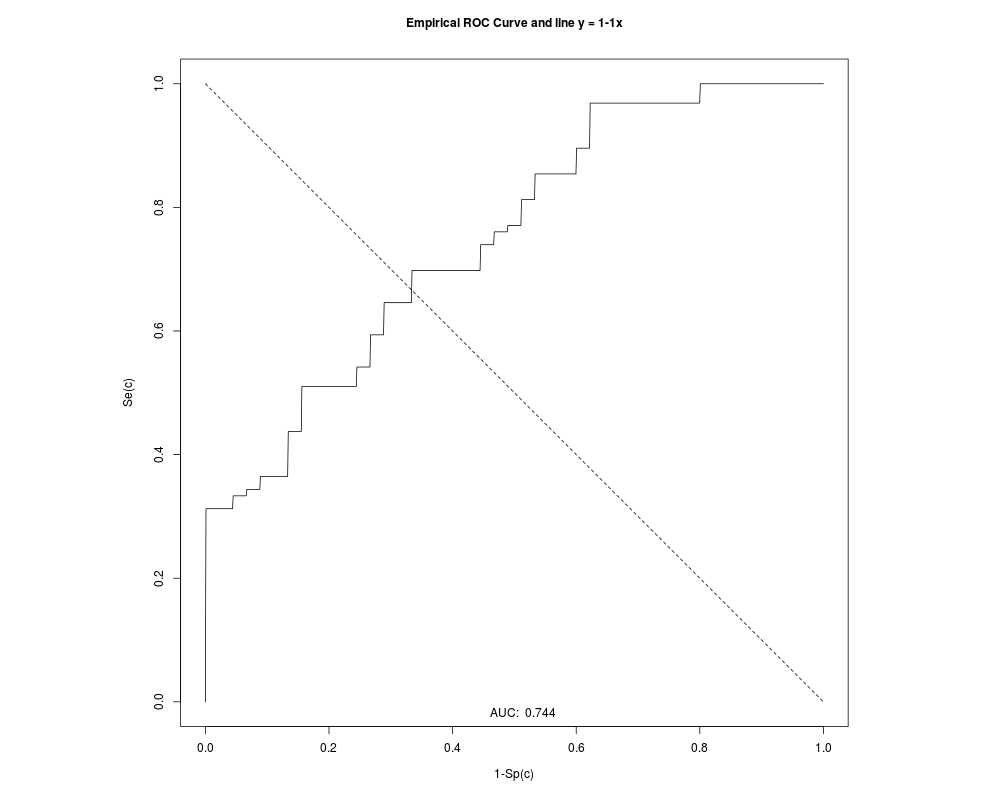
plot(gsym.point.GPQ.elastase)

Results

R version 3.3.1 (2016-06-21) -- "Bug in Your Hair"
Copyright (C) 2016 The R Foundation for Statistical Computing
Platform: x86_64-pc-linux-gnu (64-bit)

R is free software and comes with ABSOLUTELY NO WARRANTY.
You are welcome to redistribute it under certain conditions.
Type 'license()' or 'licence()' for distribution details.

R is a collaborative project with many contributors.
Type 'contributors()' for more information and
'citation()' on how to cite R or R packages in publications.

Type 'demo()' for some demos, 'help()' for on-line help, or
'help.start()' for an HTML browser interface to help.
Type 'q()' to quit R.

> library(GsymPoint)
Loading required package: truncnorm
Loading required package: Rsolnp
> png(filename="/home/ddbj/snapshot/RGM3/R_CC/result/GsymPoint/plot.gsym.point.Rd_%03d_medium.png", width=480, height=480)
> ### Name: plot.gsym.point
> ### Title: Default plotting of a gsym.point object
> ### Aliases: plot.gsym.point
> 
> ### ** Examples
> 
> library(GsymPoint)
> 
> data(melanoma)
> 
> ###########################################################
> # Generalized Pivotal Quantity Method ("GPQ"): 
> ###########################################################
> 
> gsym.point.GPQ.melanoma<-gsym.point(methods = "GPQ", data = melanoma,
+ marker = "X", status = "group", tag.healthy = 0, categorical.cov = NULL, 
+ CFN = 1, CFP = 1, control = control.gsym.point(),confidence.level = 0.95, 
+ trace = FALSE, seed = FALSE, value.seed = 3)
> 
> plot(gsym.point.GPQ.melanoma)
> 
> 
> data(prostate)
> 
> ###########################################################
> # Generalized Pivotal Quantity Method ("GPQ"): 
> ###########################################################
> 
> gsym.point.GPQ.prostate <- gsym.point (methods = "GPQ", data = prostate,
+ marker = "marker", status = "status", tag.healthy = 0, categorical.cov = NULL, 
+ CFN = 1, CFP = 1, control = control.gsym.point(), confidence.level = 0.95, 
+ trace = FALSE, seed = FALSE, value.seed = 3)
> 
> plot(gsym.point.GPQ.prostate)
> 
> 
> data(elastase)
> 
> ###########################################################
> # Generalized Pivotal Quantity Method ("GPQ"): 
> ###########################################################
> 
> gsym.point.GPQ.elastase <- gsym.point(methods = "GPQ", data = elastase, 
+ marker = "elas", status = "status", tag.healthy = 0, categorical.cov = NULL, 
+ CFN = 1, CFP = 1, control = control.gsym.point(), confidence.level = 0.95, 
+ trace = FALSE, seed = FALSE, value.seed = 3) 
According to the Shapiro-Wilk normality test, the original marker 
can not be considered normally distributed in both groups.
After transforming the marker using the Box-Cox transformation 
estimate the Shapiro-Wilk normality test indicates that the 
transformed marker can not be considered normally distributed 
in both groups. 
Therefore, the results obtained with the GPQ method may not be 
reliable. You must use the EL method instead.

Box-Cox lambda estimate = 0.1136 

Shapiro-Wilk test p-values
                           Group 0 Group 1
Original marker             0.0746  0.0091
Box-Cox transformed marker  0.0000  0.0793
> 
> plot(gsym.point.GPQ.elastase)
> 
> 
> 
> 
> 
> 
> dev.off()
null device 
          1 
>