Highest (Posterior) Density Interval

Description

Calculate the highest density interval (HDI) for a probability distribution for a given probability mass. This is often applied to a Bayesian posterior distribution and is then termed "highest posterior density interval", but can be applied to any distribution, including priors.

The function is an S3 generic, with methods for a range of input objects.

Usage

hdi(object, credMass = 0.95, ...)

## Default S3 method:
hdi(object, credMass = 0.95, ...)

## S3 method for class 'function'
hdi(object, credMass = 0.95, tol, ...)

## S3 method for class 'matrix'
hdi(object, credMass = 0.95, ...)

## S3 method for class 'data.frame'
hdi(object, credMass = 0.95, ...)

## S3 method for class 'list'
hdi(object, credMass = 0.95, ...)

## S3 method for class 'density'
hdi(object, credMass = 0.95, allowSplit=FALSE, ...)

## S3 method for class 'mcmc'
hdi(object, credMass = 0.95, ...)  

## S3 method for class 'mcmc.list'
hdi(object, credMass = 0.95, ...)  

## S3 method for class 'mcarray'
hdi(object, credMass = 0.95, ...)  

## S3 method for class 'bugs'
hdi(object, credMass = 0.95, ...)  

## S3 method for class 'jagsUI'
hdi(object, credMass = 0.95, ...)  

## S3 method for class 'rjags'
hdi(object, credMass = 0.95, ...)  

## S3 method for class 'runjags'
hdi(object, credMass = 0.95, ...)  

Arguments

Details

The HDI is the interval which contains the required mass such that all points within the interval have a higher probability density than points outside the interval.

In contrast, a symmetric density interval defined by (eg.) the 10% and 90% quantiles may include values with lower probability than those excluded.

For a distribution that is not severely multimodal, the HDI is the narrowest interval containing the specified mass, and the hdi function actually returns the narrowest interval. This does not always work properly for multimodel densities, where the HDI may be discontinuous (the horizontal black line in the Figure below). The single interval returned by hdi (the blue line) may incorrectly include values between the modes with low probability density. The density method with allowSplit = TRUE gives separate limits for discontinuous HDIs.

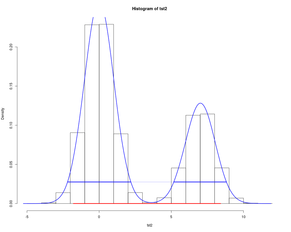
The default method expects a vector representing draws from the target distribution, such as is produced by an MCMC process. Missing values are silently ignored; if the vector has no non-missing values, NAs are returned.

The matrix and data.frame methods expect an object with vectors of the above type for each parameter in columns. The result is a matrix with parameters in columns and rows with the upper and lower limits of the HDI.

The list method is a wrapper for lapply(object, hdi, ...). It is intended for output from rjags::jags.samples which returns a list of mcarray objects.

The mcmc.list, mcmc and mcarray methods expect objects of the respective types as defined in package coda.

The packages R2winbugs and R2openbugs produce bugs objects; R2jags produces rjags; jagsUI produces jagsUI; runjags produces runjags. For the rjags package, rjags::coda.samples produces a mcmc.list object and rjags::jags.samples produces a list of mcarray objects.

None of the above use interpolation: the values returned correspond to specific values in the data object, and will be conservative (ie, too wide rather than too narrow). Results thus depend on the random draws, and will be unstable if few values are provided. For a 95% HDI, 10,000 independent draws are recommended; a smaller number will be adequate for a 80% HDI, many more for a 99% HDI.

The function method requires the name for the inverse cumulative density function (ICDF) of the distribution; standard R functions for this have a q- prefix, eg. qbeta. Arguments required by the ICDF must be specified by their (abbreviated) names; see the examples.

Value

a vector of length 2 or a 2-row matrix with the lower and upper limits of the HDI, with an attribute "credMass".

The density method with allowSplit=TRUE produces a matrix with a row for each component of a discontinuous HDI and columns for begin and end. It has an additional attribute "height" giving the probability density at the limits of the HDI.

Author(s)

Mike Meredith and John Krushke. Code for hdi.function based on hpd by Greg Snow, corrected by John Kruschke.

References

Kruschke, J. K. 2011. Doing Bayesian data analysis: a tutorial with R and BUGS. Elsevier, Amsterdam, section 3.3.5.

Examples

# for a vector:
tst <- rgamma(1e5, 2.5, 2)
hdi(tst)
hdi(tst, credMass=0.8)
# For comparison, the symmetrical 80% CrI:
quantile(tst, c(0.1,0.9))

# for a density:
dens <- density(tst)
hdi(dens, credMass=0.8)

# Now a data frame:
tst <- data.frame(mu = rnorm(1e4, 4, 1), sigma = rlnorm(1e4))
hdi(tst, 0.8)
apply(tst, 2, quantile, c(0.1,0.9))
tst$txt <- LETTERS[1:25]
hdi(tst, 0.8)

# For a function:
hdi(qgamma, 0.8, shape=2.5, rate=2)
# and the symmetrical 80% CrI:
qgamma(c(0.1, 0.9), 2.5, 2)

# A severely bimodal distribution:
tst2 <- c(rnorm(1e5), rnorm(5e4, 7))
hist(tst2, freq=FALSE)
(hdiMC <- hdi(tst2))
segments(hdiMC[1], 0, hdiMC[2], 0, lwd=3, col='red')
# This is a valid 95% CrI, but not a Highest Density Interval

dens2 <- density(tst2)
lines(dens2, lwd=2, col='blue')
(hdiD1 <- hdi(dens2))  # default allowSplit = FALSE; note the warning
(ht <- attr(hdiD1, "height"))
segments(hdiD1[1], ht, hdiD1[2], ht, lty=3, col='blue')
(hdiD2 <- hdi(dens2, allowSplit=TRUE))
segments(hdiD2[, 1], ht, hdiD2[, 2], ht, lwd=3, col='blue')
# This is the correct 95% HDI.

Results

R version 3.3.1 (2016-06-21) -- "Bug in Your Hair"
Copyright (C) 2016 The R Foundation for Statistical Computing
Platform: x86_64-pc-linux-gnu (64-bit)

R is free software and comes with ABSOLUTELY NO WARRANTY.
You are welcome to redistribute it under certain conditions.
Type 'license()' or 'licence()' for distribution details.

R is a collaborative project with many contributors.
Type 'contributors()' for more information and
'citation()' on how to cite R or R packages in publications.

Type 'demo()' for some demos, 'help()' for on-line help, or
'help.start()' for an HTML browser interface to help.
Type 'q()' to quit R.

> library(HDInterval)
> png(filename="/home/ddbj/snapshot/RGM3/R_CC/result/HDInterval/hdi.Rd_%03d_medium.png", width=480, height=480)
> ### Name: hdi
> ### Title: Highest (Posterior) Density Interval
> ### Aliases: HDInterval hdi hdi.default hdi.function hdi.matrix
> ###   hdi.data.frame hdi.list hdi.density hdi.mcmc hdi.mcarray
> ###   hdi.mcmc.list hdi.bugs hdi.jagsUI hdi.rjags hdi.runjags
> ### Keywords: methods htest
> 
> ### ** Examples
> 
> # for a vector:
> tst <- rgamma(1e5, 2.5, 2)
> hdi(tst)
     lower      upper 
0.07421291 2.77720536 
attr(,"credMass")
[1] 0.95
> hdi(tst, credMass=0.8)
    lower     upper 
0.1870523 1.8901953 
attr(,"credMass")
[1] 0.8
> # For comparison, the symmetrical 80% CrI:
> quantile(tst, c(0.1,0.9))
      10%       90% 
0.4056557 2.3024642 
> 
> # for a density:
> dens <- density(tst)
> hdi(dens, credMass=0.8)
   lower    upper 
0.206056 1.913838 
attr(,"credMass")
[1] 0.8
attr(,"height")
[1] 0.2393585
> 
> # Now a data frame:
> tst <- data.frame(mu = rnorm(1e4, 4, 1), sigma = rlnorm(1e4))
> hdi(tst, 0.8)
            mu      sigma
lower 2.776759 0.06131656
upper 5.358374 2.30314266
attr(,"credMass")
[1] 0.8
> apply(tst, 2, quantile, c(0.1,0.9))
          mu     sigma
10% 2.726329 0.2721758
90% 5.314381 3.6120315
> tst$txt <- LETTERS[1:25]
> hdi(tst, 0.8)
            mu      sigma txt
lower 2.776759 0.06131656  NA
upper 5.358374 2.30314266  NA
attr(,"credMass")
[1] 0.8
> 
> # For a function:
> hdi(qgamma, 0.8, shape=2.5, rate=2)
    lower     upper 
0.1947158 1.9053925 
attr(,"credMass")
[1] 0.8
> # and the symmetrical 80% CrI:
> qgamma(c(0.1, 0.9), 2.5, 2)
[1] 0.402577 2.309089
> 
> # A severely bimodal distribution:
> tst2 <- c(rnorm(1e5), rnorm(5e4, 7))
> hist(tst2, freq=FALSE)
> (hdiMC <- hdi(tst2))
    lower     upper 
-1.835687  8.378939 
attr(,"credMass")
[1] 0.95
> segments(hdiMC[1], 0, hdiMC[2], 0, lwd=3, col='red')
> # This is a valid 95% CrI, but not a Highest Density Interval
> 
> dens2 <- density(tst2)
> lines(dens2, lwd=2, col='blue')
> (hdiD1 <- hdi(dens2))  # default allowSplit = FALSE; note the warning
    lower     upper 
-1.916874  8.462495 
attr(,"credMass")
[1] 0.95
attr(,"height")
[1] 0.02838018
Warning message:
In hdi.density(dens2) : The HDI is discontinuous but allowSplit = FALSE;
    the result is a valid CrI but not HDI.
> (ht <- attr(hdiD1, "height"))
[1] 0.02838018
> segments(hdiD1[1], ht, hdiD1[2], ht, lty=3, col='blue')
> (hdiD2 <- hdi(dens2, allowSplit=TRUE))
         begin      end
[1,] -2.172105 2.183828
[2,]  5.212562 8.819818
attr(,"credMass")
[1] 0.95
attr(,"height")
[1] 0.02838018
> segments(hdiD2[, 1], ht, hdiD2[, 2], ht, lwd=3, col='blue')
> # This is the correct 95% HDI.
> 
> 
> 
> 
> 
> dev.off()
null device 
          1 
>