Plot a chisquare or a F-curve. Shade a region for
rejection region or do-not-reject region. F.observed and
chisq.observed plots a vertical line with arrowhead markers at
the location of the observed xbar and outlines the area corresponding
to the p-value.
Initial settings for xlim, ylim.
The defaults are calculated for the degrees of freedom.
df, df1, df2, ncp, log.p
Degrees of freedom,
non-centrality parameter, probabilities are given as log(p).
See pchisq and pf.
alpha
Probability of a Type I error. alpha is a vector
of
one or two values. If one value, it is the right alpha. If two values,
they are the c(left.alpha, right.alpha).
critical.values
Critical values. Initial values correspond
to the specified alpha levels.
A scalar value implies a one-sided test on the right side.
A vector of two values
implies a two-sided test.
main.in, ylab.in
Main title, default ylab.
shade
Valid values for shade are "right", "left", "inside", "outside", "none".
Default is "right" for one-sided critical.values and "outside"
for two-sided critical values.
col
color of the shaded region and the area of the shaded region.
shaded.area
Numerical value of the area. This value may
be cumulated over two calls to the function (one call for left, one
call for right).
The shaded.area is the return value of the function.
The calling program is responsible for the
cumulation.
display.obs
Logical. If TRUE, print the numerical value
of the observed value, plot a vertical abline at the value,
and use it for showing the p-value.
If FALSE, don't print or plot the observed value; just use it
for showing the p-value.
f,chisq
Values used to draw curve. Replace them if more
resolution is needed.
f.obs, chisq.obs
Observed values of statistic. p-values are
calculated for these values.
R version 3.3.1 (2016-06-21) -- "Bug in Your Hair"
Copyright (C) 2016 The R Foundation for Statistical Computing
Platform: x86_64-pc-linux-gnu (64-bit)
R is free software and comes with ABSOLUTELY NO WARRANTY.
You are welcome to redistribute it under certain conditions.
Type 'license()' or 'licence()' for distribution details.
R is a collaborative project with many contributors.
Type 'contributors()' for more information and
'citation()' on how to cite R or R packages in publications.
Type 'demo()' for some demos, 'help()' for on-line help, or
'help.start()' for an HTML browser interface to help.
Type 'q()' to quit R.
> library(HH)
Loading required package: lattice
Loading required package: grid
Loading required package: latticeExtra
Loading required package: RColorBrewer
Loading required package: multcomp
Loading required package: mvtnorm
Loading required package: survival
Loading required package: TH.data
Loading required package: MASS
Attaching package: 'TH.data'
The following object is masked from 'package:MASS':
geyser
Loading required package: gridExtra
> png(filename="/home/ddbj/snapshot/RGM3/R_CC/result/HH/F.curve.Rd_%03d_medium.png", width=480, height=480)
> ### Name: F.curve
> ### Title: plot a chisquare or a F-curve.
> ### Aliases: chisq.curve chisq.observed chisq.setup F.curve F.observed
> ### F.setup
> ### Keywords: aplot hplot distribution
>
> ### ** Examples
>
> old.omd <- par(omd=c(.05,.88, .05,1))
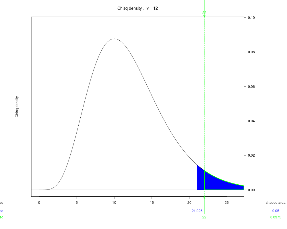
> chisq.setup(df=12)
> chisq.curve(df=12, col='blue')
> chisq.observed(22, df=12)
> par(old.omd)
>
> old.omd <- par(omd=c(.05,.88, .05,1))
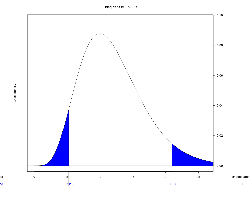
> chisq.setup(df=12)
> chisq.curve(df=12, col='blue', alpha=c(.05, .05))
> par(old.omd)
>
> old.omd <- par(omd=c(.05,.88, .05,1))
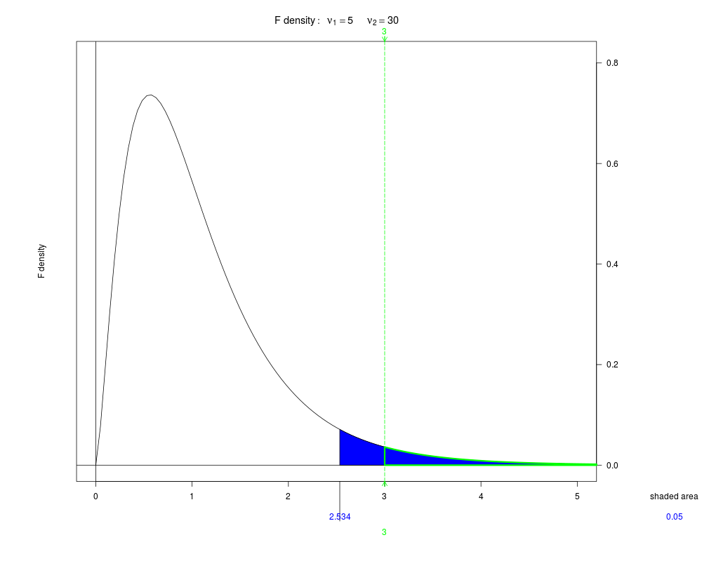
> F.setup(df1=5, df2=30)
> F.curve(df1=5, df2=30, col='blue')
> F.observed(3, df1=5, df2=30)
> par(old.omd)
>
> old.omd <- par(omd=c(.05,.88, .05,1))
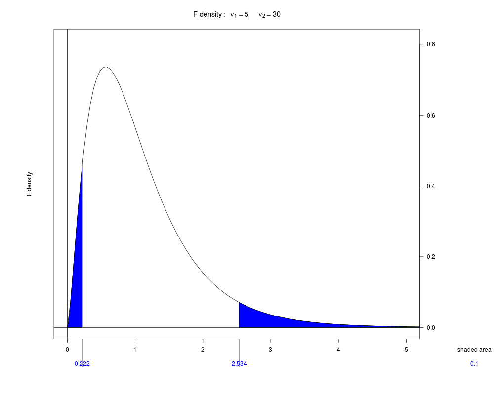
> F.setup(df1=5, df2=30)
> F.curve(df1=5, df2=30, col='blue', alpha=c(.05, .05))
> par(old.omd)
>
>
>
>
>
>
> dev.off()
null device
1
>
 .
.