Supported by Dr. Osamu Ogasawara and  . . |
|
Last data update: 2014.03.03 |
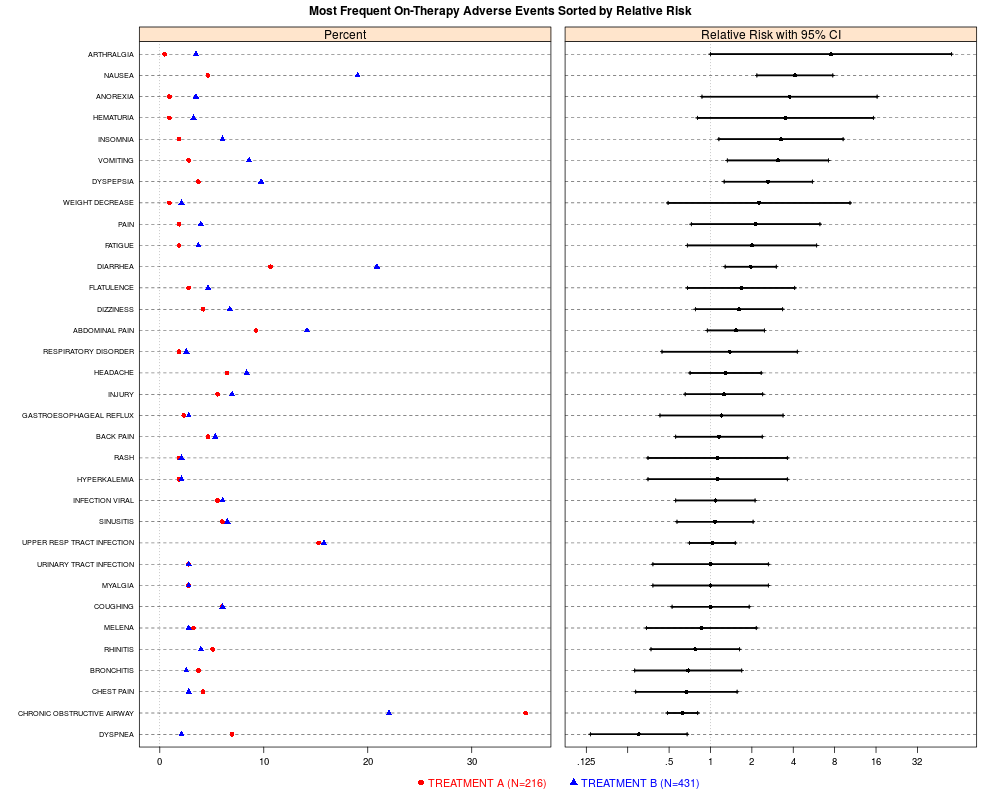
AE (Adverse Events) dotplot of incidence and relative riskDescriptionA two-panel display of the most frequently occurring AEs in the active arm of a clinical study. The first panel displays their incidence by treatment group, with different symbols for each group. The second panel displays the relative risk of an event on the active arm relative to the placebo arm, with 95% confidence intervals for a 2x2 table. By default, the AEs are ordered by relative risk so that events with the largest increases in risk for the active treatment are prominent at the top of the display. See the Details section for information on changing the sort order. Usage
ae.dotplot(ae, ...)

ae.dotplot.long(xr,
                A.name = levels(xr$RAND)[1], B.name = levels(xr$RAND)[2],
                col.AB = c("red","blue"), pch.AB = c(16, 17),
                main.title = paste("Most Frequent On-Therapy Adverse Events",
                                   "Sorted by Relative Risk"),
                main.cex = 1,
                cex.AB.points = NULL, cex.AB.y.scale = 0.6,
                position.left = c(0, 0, 0.7, 1), position.right = c(0.61, 0, 0.98, 1),
                key.y = -0.2, CI.percent=95)

logrelrisk(ae, A.name, B.name, crit.value=1.96)

panel.ae.leftplot(x, y, groups, col.AB, ...)

panel.ae.rightplot(x, y, ..., lwd=6, lower, upper, cex=.7)

panel.ae.dotplot(x, y, groups, ..., col.AB, pch.AB, lower, upper) ## R only

aeReshapeToLong(aewide)
Arguments
DetailsThe second panel shows relative risk of an event on the active arm (treatment B) relative to the placebo arm (treatment A), with 95% confidence intervals for a 2x2 table. Confidence intervals on the log relative risk are calculated using the asymptotic standard error formula given as Equation 3.18 in Agresti A., Categorical Data Analysis. Wiley: New York, 1990. By default the Value
Author(s)Richard M. Heiberger <rmh@temple.edu> ReferencesOhad Amit, Richard M. Heiberger, and Peter W. Lane. (2008) “Graphical Approaches to the Analysis of Safety Data from Clinical Trials”. Pharmaceutical Statistics, 7, 1, 20–35. http://www3.interscience.wiley.com/journal/114129388/abstract Examples
## variable names in the input data.frame aeanonym
## RAND treatment as randomized
## PREF adverse event symptom name
## SN number of patients in treatment group
## SAE number of patients in each group for whom the event PREF was observed
##
## Input sort order is PREF/RAND
data(aeanonym)
head(aeanonym)
## Calculate log relative risk and confidence intervals (95% by default).
## logrelrisk sets the sort order for PREF to match the relative risk.
aeanonymr <- logrelrisk(aeanonym) ## sorts by relative risk
head(aeanonymr)
## construct and print plot on current graphics device
ae.dotplot(aeanonymr,
A.name="TREATMENT A (N=216)",
B.name="TREATMENT B (N=431)")
## export.eps(h2("stdt/figure/aerelrisk.eps"))
## This looks great on screen and exports badly to eps.
## We recommend drawing this plot directly to the postscript device:
##
## trellis.device(postscript, color=TRUE, horizontal=TRUE,
## colors=ps.colors.rgb[
## c("black", "blue", "red", "green",
## "yellow", "cyan","magenta","brown"),],
## onefile=FALSE, print.it=FALSE,
## file=h2("stdt/figure/aerelrisk.ps"))
## ae.dotplot(aeanonymr,
## A.name="TREATMENT A (N=216)",
## B.name="TREATMENT B (N=431)")
## dev.off()
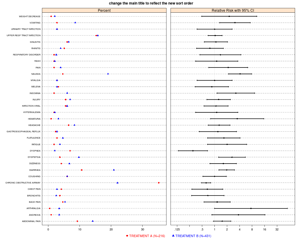
## To change the sort order, redefine the PREF factor.
## For this example, to plot alphabetically, use the statement
aeanonymr$PREF <- ordered(aeanonymr$PREF, levels=sort(levels(aeanonymr$PREF)))
ae.dotplot(aeanonymr,
A.name="TREATMENT A (N=216)",
B.name="TREATMENT B (N=431)",
main.title="change the main title to reflect the new sort order")
## Not run:
## to restore the order back to the default, use
relrisk <- aeanonymr[seq(1, nrow(aeanonymr), 2), "relrisk"]
PREF <- unique(aeanonymr$PREF)
aeanonymr$PREF <- ordered(aeanonymr$PREF, levels=PREF[order(relrisk)])
ae.dotplot(aeanonymr,
A.name="TREATMENT A (N=216)",
B.name="TREATMENT B (N=431)",
main.title="back to the original sort order")
## smaller artifical example with the wide format
aewide <- data.frame(Event=letters[1:6],
N.A=c(50,50,50,50,50,50),
N.B=c(90,90,90,90,90,90),
AE.A=2*(1:6),
AE.B=1:6)
aewtol <- aeReshapeToLong(aewide)
xr <- logrelrisk(aewtol)
ae.dotplot(xr)
## End(Not run)
Results
R version 3.3.1 (2016-06-21) -- "Bug in Your Hair"
Copyright (C) 2016 The R Foundation for Statistical Computing
Platform: x86_64-pc-linux-gnu (64-bit)

R is free software and comes with ABSOLUTELY NO WARRANTY.
You are welcome to redistribute it under certain conditions.
Type 'license()' or 'licence()' for distribution details.

R is a collaborative project with many contributors.
Type 'contributors()' for more information and
'citation()' on how to cite R or R packages in publications.

Type 'demo()' for some demos, 'help()' for on-line help, or
'help.start()' for an HTML browser interface to help.
Type 'q()' to quit R.

> library(HH)
Loading required package: lattice
Loading required package: grid
Loading required package: latticeExtra
Loading required package: RColorBrewer
Loading required package: multcomp
Loading required package: mvtnorm
Loading required package: survival
Loading required package: TH.data
Loading required package: MASS

Attaching package: 'TH.data'

The following object is masked from 'package:MASS':

    geyser

Loading required package: gridExtra
> png(filename="/home/ddbj/snapshot/RGM3/R_CC/result/HH/ae.dotplot.Rd_%03d_medium.png", width=480, height=480)
> ### Name: ae.dotplot
> ### Title: AE (Adverse Events) dotplot of incidence and relative risk
> ### Aliases: ae.dotplot AE.dotplot ae.dotplot.long aeReshapeToLong
> ###   panel.ae.leftplot panel.ae.rightplot panel.ae.dotplot logrelrisk
> ### Keywords: hplot htest
>
> ### ** Examples
>
> ## variable names in the input data.frame aeanonym
> ## RAND   treatment as randomized
> ## PREF   adverse event symptom name
> ## SN     number of patients in treatment group
> ## SAE    number of patients  in each group for whom the event PREF was observed
> ##
> ## Input sort order is PREF/RAND
>
> data(aeanonym)
> head(aeanonym)
         RAND         PREF SAE  SN OrgSys
1 TREATMENT A      DYSPNEA  15 216   Resp
2 TREATMENT B      DYSPNEA   9 431   Resp
3 TREATMENT A HYPERKALEMIA   4 216   Misc
4 TREATMENT B HYPERKALEMIA   9 431   Misc
5 TREATMENT A         RASH   4 216   Misc
6 TREATMENT B         RASH   9 431   Misc
>
> ## Calculate log relative risk and confidence intervals (95% by default).
> ## logrelrisk sets the sort order for PREF to match the relative risk.
> aeanonymr <- logrelrisk(aeanonym) ## sorts by relative risk
> head(aeanonymr)
          RAND           PREF SAE  SN OrgSys        PCT  relrisk logrelrisk
57 TREATMENT A ABDOMINAL PAIN  20 216     GI  9.2592593 1.528538  0.4243119
58 TREATMENT B ABDOMINAL PAIN  61 431     GI 14.1531323 1.528538  0.4243119
25 TREATMENT A       ANOREXIA   2 216     GI  0.9259259 3.758701  1.3240733
26 TREATMENT B       ANOREXIA  15 431     GI  3.4802784 3.758701  1.3240733
27 TREATMENT A     ARTHRALGIA   1 216   Pain  0.4629630 7.517401  2.0172205
28 TREATMENT B     ARTHRALGIA  15 431   Pain  3.4802784 7.517401  2.0172205
   ase.logrelrisk logrelriskCI.lower logrelriskCI.upper relriskCI.lower
57      0.2438106      -0.0535569430          0.9021808       0.9478520
58      0.2438106      -0.0535569430          0.9021808       0.9478520
25      0.7481423      -0.1422855049          2.7904322       0.8673736
26      0.7481423      -0.1422855049          2.7904322       0.8673736
27      1.0294255      -0.0004534531          4.0348945       0.9995466
28      1.0294255      -0.0004534531          4.0348945       0.9995466
   relriskCI.upper
57        2.464973
58        2.464973
25       16.288058
26       16.288058
27       56.536955
28       56.536955
>
> ## construct and print plot on current graphics device
> ae.dotplot(aeanonymr,
+            A.name="TREATMENT A (N=216)",
+            B.name="TREATMENT B (N=431)")
> ## export.eps(h2("stdt/figure/aerelrisk.eps"))
> ## This looks great on screen and exports badly to eps.
> ## We recommend drawing this plot directly to the postscript device:
> ##
> ## trellis.device(postscript, color=TRUE, horizontal=TRUE,
> ##                colors=ps.colors.rgb[
> ##                  c("black", "blue", "red", "green",
> ##                    "yellow", "cyan","magenta","brown"),],
> ##                onefile=FALSE, print.it=FALSE,
> ##                file=h2("stdt/figure/aerelrisk.ps"))
> ## ae.dotplot(aeanonymr,
> ##            A.name="TREATMENT A (N=216)",
> ##            B.name="TREATMENT B (N=431)")
> ## dev.off()
>
> ## To change the sort order, redefine the PREF factor.
> ## For this example, to plot alphabetically, use the statement
> aeanonymr$PREF <- ordered(aeanonymr$PREF, levels=sort(levels(aeanonymr$PREF)))
> ae.dotplot(aeanonymr,
+            A.name="TREATMENT A (N=216)",
+            B.name="TREATMENT B (N=431)",
+            main.title="change the main title to reflect the new sort order")
>
> ## Not run:
> ##D ## to restore the order back to the default, use
> ##D relrisk <- aeanonymr[seq(1, nrow(aeanonymr), 2), "relrisk"]
> ##D PREF <- unique(aeanonymr$PREF)
> ##D aeanonymr$PREF <- ordered(aeanonymr$PREF, levels=PREF[order(relrisk)])
> ##D ae.dotplot(aeanonymr,
> ##D            A.name="TREATMENT A (N=216)",
> ##D            B.name="TREATMENT B (N=431)",
> ##D            main.title="back to the original sort order")
> ##D
> ##D ## smaller artifical example with the wide format
> ##D aewide <- data.frame(Event=letters[1:6],
> ##D                      N.A=c(50,50,50,50,50,50),
> ##D                      N.B=c(90,90,90,90,90,90),
> ##D                      AE.A=2*(1:6),
> ##D                      AE.B=1:6)
> ##D aewtol <- aeReshapeToLong(aewide)
> ##D xr <- logrelrisk(aewtol)
> ##D ae.dotplot(xr)
> ## End(Not run)
>
>
>
>
>
> dev.off()
null device
          1
>
|