Supported by Dr. Osamu Ogasawara and  . . |
|
Last data update: 2014.03.03 |
Compute and plot oneway analysis of covarianceDescriptionCompute and plot oneway analysis of covariance.
The result object is an Usage
ancova(formula, data.in = NULL, ...,
       x, groups, transpose = FALSE,
       display.plot.command = FALSE,
       superpose.level.name = "superpose",
       ignore.groups = FALSE, ignore.groups.name = "ignore.groups",
       blocks, blocks.pch = letters[seq(levels(blocks))],
       layout, between, main,
       pch=trellis.par.get()$superpose.symbol$pch)

panel.ancova(x, y, subscripts, groups,
 transpose = FALSE, ...,
 coef, contrasts, classes,
 ignore.groups, blocks, blocks.pch, blocks.cex, pch)

## The following are ancova methods for generic functions.
## S3 method for class 'ancova'
anova(object, ...)

## S3 method for class 'ancova'
predict(object, ...)

## S3 method for class 'ancova'
print(x, ...) ## prints the anova(x) and the trellis attribute

## S3 method for class 'ancova'
model.frame(formula, ...)

## S3 method for class 'ancova'
summary(object, ...)

## S3 method for class 'ancova'
plot(x, y, ...) ## standard lm plot.  y is always ignored.

## S3 method for class 'ancova'
coef(object, ...)
Arguments
object. The functions using this argument are methods for the similarly named generic functions.
Details The Value The result object is an Author(s)Richard M. Heiberger <rmh@temple.edu> ReferencesHeiberger, Richard M. and Holland, Burt (2004b). Statistical Analysis and Data Display: An Intermediate Course with Examples in S-Plus, R, and SAS. Springer Texts in Statistics. Springer. ISBN 0-387-40270-5. See Also
Examples
data(hotdog)
## y ~ x ## constant line across all groups
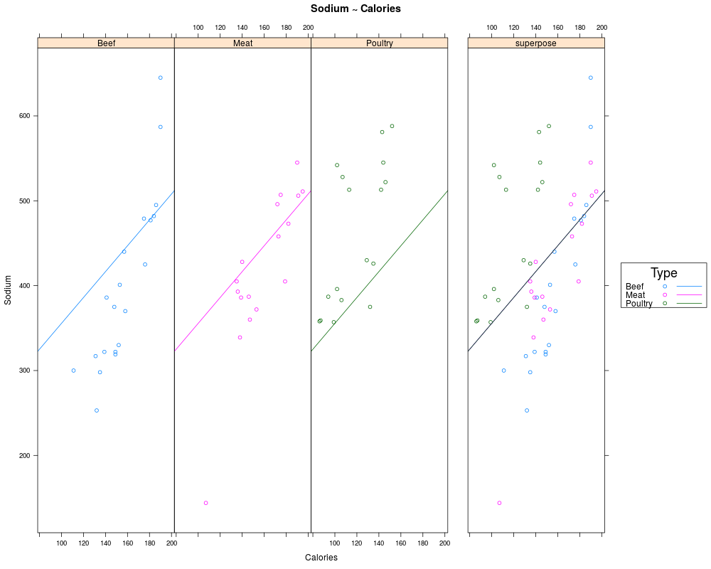
ancova(Sodium ~ Calories, data=hotdog, groups=Type)
## y ~ a ## different horizontal line in each group
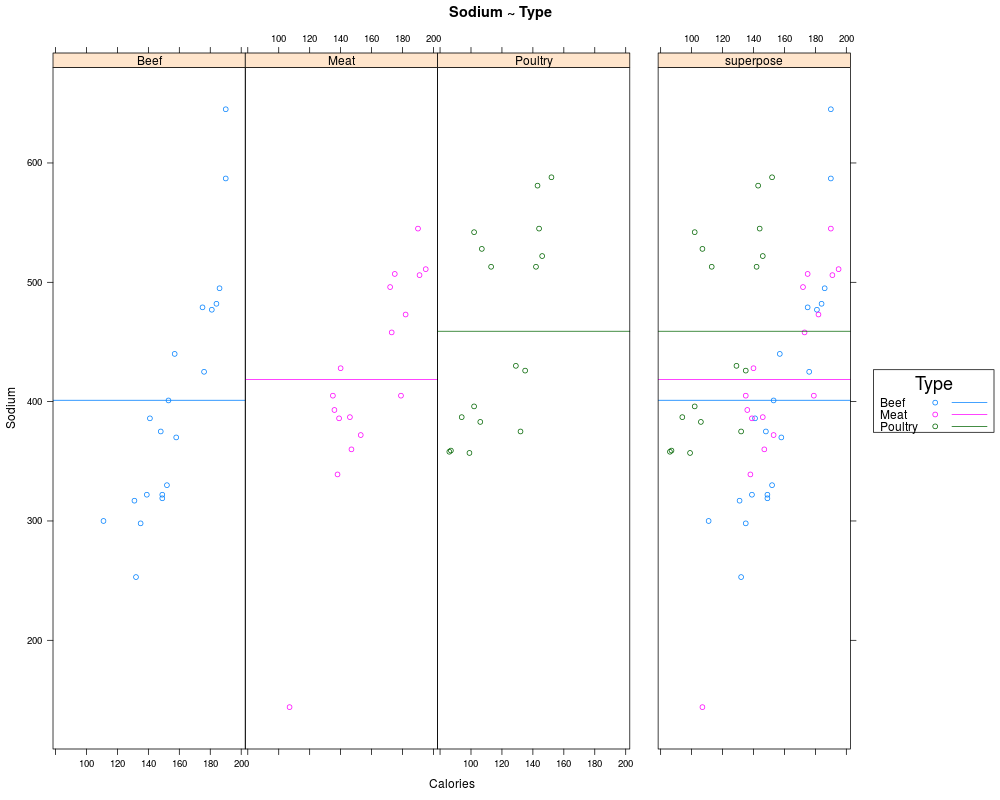
ancova(Sodium ~ Type, data=hotdog, x=Calories)
## This is the usual usage
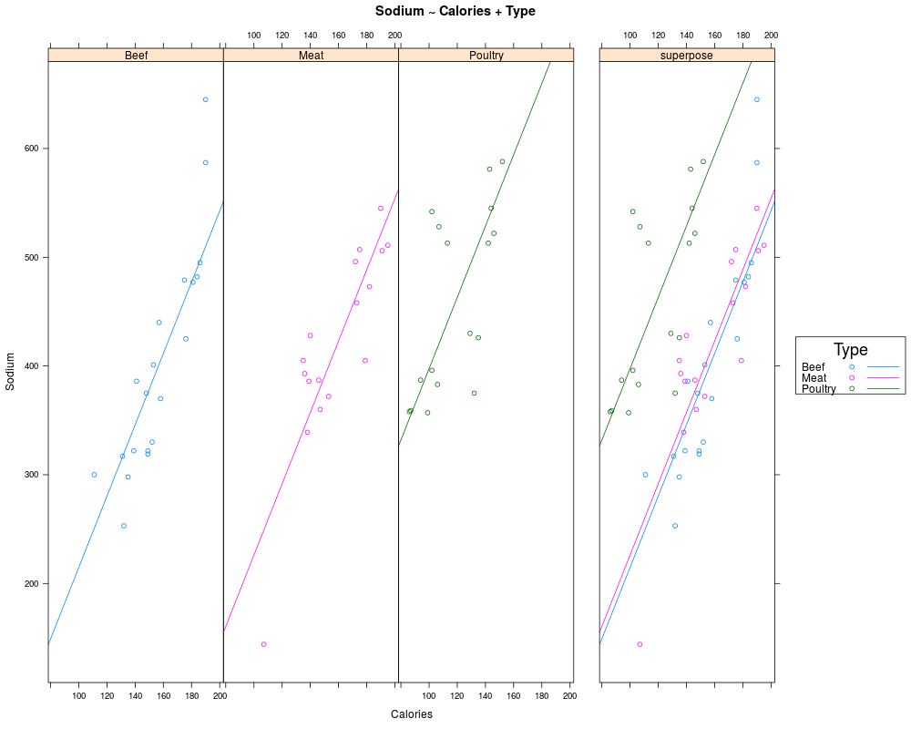
## y ~ x + a or y ~ a + x ## constant slope, different intercepts
ancova(Sodium ~ Calories + Type, data=hotdog)
ancova(Sodium ~ Type + Calories, data=hotdog)
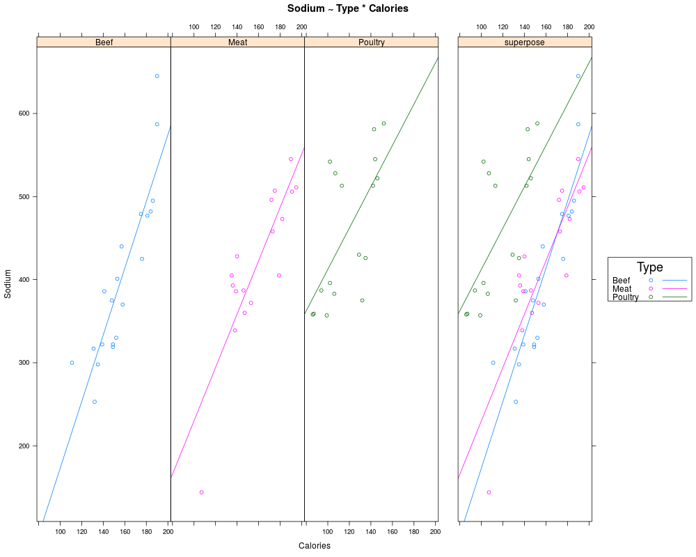
## y ~ x * a or y ~ a * x ## different slopes, and different intercepts
ancova(Sodium ~ Calories * Type, data=hotdog)
ancova(Sodium ~ Type * Calories, data=hotdog)
## y ~ a * x ## save the object and print the trellis graph
hotdog.ancova <- ancova(Sodium ~ Type * Calories, data=hotdog)
attr(hotdog.ancova, "trellis")
## label points in the panels by the value of the block factor
data(apple)
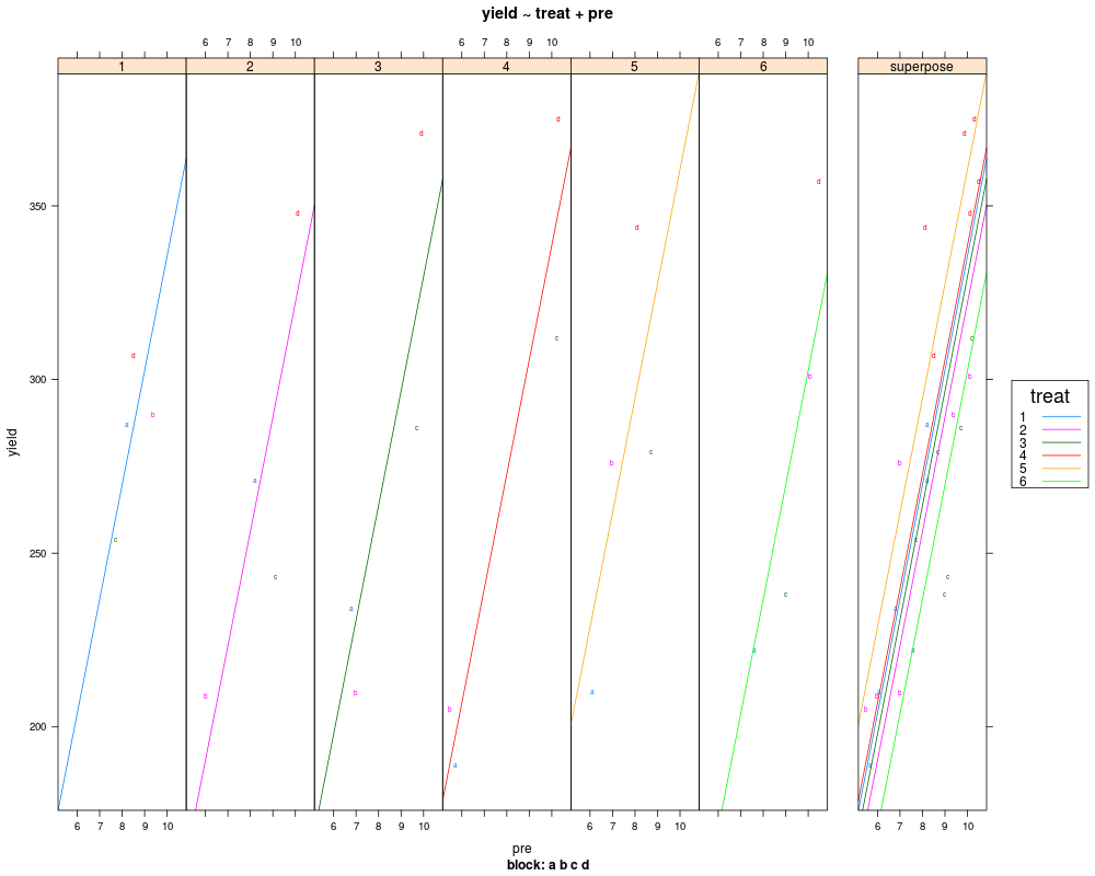
ancova(yield ~ treat + pre, data=apple, blocks=block)
## Please see
## demo("ancova")
## for a composite graph illustrating the four models listed above.
Results
R version 3.3.1 (2016-06-21) -- "Bug in Your Hair"
Copyright (C) 2016 The R Foundation for Statistical Computing
Platform: x86_64-pc-linux-gnu (64-bit)

R is free software and comes with ABSOLUTELY NO WARRANTY.
You are welcome to redistribute it under certain conditions.
Type 'license()' or 'licence()' for distribution details.

R is a collaborative project with many contributors.
Type 'contributors()' for more information and
'citation()' on how to cite R or R packages in publications.

Type 'demo()' for some demos, 'help()' for on-line help, or
'help.start()' for an HTML browser interface to help.
Type 'q()' to quit R.

> library(HH)
Loading required package: lattice
Loading required package: grid
Loading required package: latticeExtra
Loading required package: RColorBrewer
Loading required package: multcomp
Loading required package: mvtnorm
Loading required package: survival
Loading required package: TH.data
Loading required package: MASS

Attaching package: 'TH.data'

The following object is masked from 'package:MASS':

    geyser

Loading required package: gridExtra
> png(filename="/home/ddbj/snapshot/RGM3/R_CC/result/HH/ancova.Rd_%03d_medium.png", width=480, height=480)
> ### Name: ancova
> ### Title: Compute and plot oneway analysis of covariance
> ### Aliases: ancova 'analysis of covariance' covariance anova.ancova
> ###   predict.ancova print.ancova model.frame.ancova summary.ancova
> ###   plot.ancova coef.ancova panel.ancova
> ### Keywords: hplot dplot models regression
>
> ### ** Examples
>
> data(hotdog)
>
> ## y ~ x                     ## constant line across all groups
> ancova(Sodium ~ Calories,     data=hotdog, groups=Type)
Analysis of Variance Table

Response: Sodium
          Df Sum Sq Mean Sq F value    Pr(>F)
Calories   1 106270  106270  14.515 0.0003693 ***
Residuals 52 380718    7321
---
Signif. codes:  0 '***' 0.001 '**' 0.01 '*' 0.05 '.' 0.1 ' ' 1
>
> ## y ~ a                     ## different horizontal line in each group
> ancova(Sodium ~            Type, data=hotdog, x=Calories)
Analysis of Variance Table

Response: Sodium
          Df Sum Sq Mean Sq F value Pr(>F)
Type       2  31739 15869.4  1.7778 0.1793
Residuals 51 455249  8926.4
>
> ## This is the usual usage
> ## y ~ x + a  or  y ~ a + x  ## constant slope, different intercepts
> ancova(Sodium ~ Calories + Type, data=hotdog)
Analysis of Variance Table

Response: Sodium
          Df Sum Sq Mean Sq F value    Pr(>F)
Calories   1 106270  106270  34.654 3.281e-07 ***
Type       2 227386  113693  37.074 1.336e-10 ***
Residuals 50 153331    3067
---
Signif. codes:  0 '***' 0.001 '**' 0.01 '*' 0.05 '.' 0.1 ' ' 1
> ancova(Sodium ~ Type + Calories, data=hotdog)
Analysis of Variance Table

Response: Sodium
          Df Sum Sq Mean Sq F value    Pr(>F)
Type       2  31739   15869  5.1749  0.009065 **
Calories   1 301917  301917 98.4526 2.089e-13 ***
Residuals 50 153331    3067
---
Signif. codes:  0 '***' 0.001 '**' 0.01 '*' 0.05 '.' 0.1 ' ' 1
>
> ## y ~ x * a  or  y ~ a * x  ## different slopes, and different intercepts
> ancova(Sodium ~ Calories * Type, data=hotdog)
Analysis of Variance Table

Response: Sodium
              Df Sum Sq Mean Sq F value    Pr(>F)
Calories       1 106270  106270 35.6885 2.747e-07 ***
Type           2 227386  113693 38.1815 1.195e-10 ***
Calories:Type  2  10402    5201  1.7466    0.1853
Residuals     48 142930    2978
---
Signif. codes:  0 '***' 0.001 '**' 0.01 '*' 0.05 '.' 0.1 ' ' 1
> ancova(Sodium ~ Type * Calories, data=hotdog)
Analysis of Variance Table

Response: Sodium
              Df Sum Sq Mean Sq  F value    Pr(>F)
Type           2  31739   15869   5.3294  0.008124 **
Calories       1 301917  301917 101.3927 2.019e-13 ***
Type:Calories  2  10402    5201   1.7466  0.185267
Residuals     48 142930    2978
---
Signif. codes:  0 '***' 0.001 '**' 0.01 '*' 0.05 '.' 0.1 ' ' 1
>
> ## y ~ a * x ## save the object and print the trellis graph
> hotdog.ancova <- ancova(Sodium ~ Type * Calories, data=hotdog)
> attr(hotdog.ancova, "trellis")
>
>
> ## label points in the panels by the value of the block factor
> data(apple)
> ancova(yield ~ treat + pre, data=apple, blocks=block)
Analysis of Variance Table

Response: yield
          Df Sum Sq Mean Sq F value    Pr(>F)
treat      5    750     150  0.1486    0.9777
pre        1  54142   54142 53.6893 1.181e-06 ***
Residuals 17  17143    1008
---
Signif. codes:  0 '***' 0.001 '**' 0.01 '*' 0.05 '.' 0.1 ' ' 1
>
> ## Please see
> ##      demo("ancova")
> ## for a composite graph illustrating the four models listed above.
>
>
>
>
>
> dev.off()
null device
          1
>
|