R Graphical Manual

Browse All

Last data update: 2014.03.03

R: Analysis of Covariance Plots

ancovaplot

R Documentation

Analysis of Covariance Plots

Description

Analysis of Covariance Plots. Any of the ancova models
y ~ x * t
y ~ t * x
y ~ x + t
y ~ t + x
y ~ x , groups=t
y ~ t, x=x
y ~ x * t, groups=b
y ~ t * x, groups=b
y ~ x + t, groups=b
y ~ t + x, groups=b

Usage

ancovaplot(object, ...)
## S3 method for class 'formula'
ancovaplot(object, data, groups=NULL, x=NULL, ...,
           formula=object,
           col=rep(tpg$col,
             length=length(levels(as.factor(groups)))),
           pch=rep(c(15,19,17,18,16,20, 0:14),
             length=length(levels(as.factor(groups)))),
           slope, intercept,
           layout=c(length(levels(cc)), 1),
           col.line=col, lty=1,
           superpose.panel=TRUE,
           between=if (superpose.panel)
                      list(x=c(rep(0, length(levels(cc))-1), 1))
                   else
                      list(x=0),
           col.by.groups=FALSE ## ignored unless groups= is specified
           )

panel.ancova.superpose(x, y, subscripts, groups,
                       slope, intercept,
                       col, pch, ...,
                       col.line, lty,
                       superpose.panel,
                       col.by.groups,
                       condition.factor,
                       groups.cc.incompatible,
                       plot.resids=FALSE,
                       print.resids=FALSE,
                       mean.x.line=FALSE,
                       col.mean.x.line="gray80")

Arguments

`formula, object`	`formula` specifying the `aov` model. The function modifies it for the `xyplot` specification.
`data`	`data.frame`
`groups`	If the treatment factor is included in the `formula`, then `groups` is not needed. By default `groups` will be set to the treatment factor, but the user may specify another factor for `groups`, usually a blocking factor. The `pch` will follow the value of `groups`. If the treatment is not included in the `formula`, then `groups` is required.
`x`	Covariate. Required by `ancovaplot.formula` if the covariate is not included in the `formula`. For `panel.ancova.superpose`, see `panel.superpose`.
`...`	Other arguments to be passed to `xyplot`.
`col, pch`	Standard lattice arguments. `pch` follows the value of `groups`. When `col.by.groups` is `TRUE`, then `col` follow the value of `groups`. When `col.by.groups` is `FALSE`, then `col` follows the value of the treatment factor, and is constant in each panel.
`slope, intercept`	Vector, the length of the number of treatment levels, containing slope and intercept of the `abline` in each panel. This is by default calculated based on the formula. The user may override each independently.
`layout, between`	Standard lattice arguments.
`col.line, lty`	Standard lattice arguments. By default, they follow the value of the treatment factor in the `formula`. `col.line` is recycled to the number of panels in the plot.
`y, subscripts`	See `panel.xyplot`.
`superpose.panel`	logical. if `TRUE` (the default), there is an additional panel on the right containing the superposition of the points and lines for all treatment levels.
`col.by.groups`	logical. See the discussion in argument `col`.
`condition.factor, groups.cc.incompatible`	These are both internal variables. `condition.factor` contains a copy of the treatment factor. `groups.cc.incompatible` is a logical which is set to `TRUE` when the `groups` argument is explicitly set by the user.
`plot.resids, print.resids, mean.x.line, col.mean.x.line`	logical, logical, logical or numeric, color name. When `plot.resids==TRUE` then vertical line segments connecting the data points and the fitted line are drawn. The other two arguments are interpreted only when `plot.resids==TRUE`. When `print.resids==TRUE` then the values of the residuals are printed on the console. When `is.numeric(mean.x.line)` then a vertical reference line is drawn at the specified value, which will normally be specified by the user as the mean of the full set of x values. The reference line will have color specified by `col.mean.x.line`.

Details

`ancova=aov specification`	`xyplot specification`	`abline`
`y ~ x * t`	`y ~ x \| t, groups=t`	`lm(y[t] ~ x[t])`	`## separate lines`
`y ~ t * x`	`y ~ x \| t, groups=t`	`lm(y[t] ~ x[t])`	`## separate lines`
`y ~ x + t`	`y ~ x \| t, groups=t`	`lm(y ~ x + t)`	`## parallel lines`
`y ~ t + x`	`y ~ x \| t, groups=t`	`lm(y ~ x + t)`	`## parallel lines`
`y ~ x , groups=t`	`y ~ x \| t, groups=t`	`lm(y ~ x)`	`## single regression line`
`y ~ t, x=x`	`y ~ x \| t, groups=t`	`mean(t)`	`## separate horizontal lines`
`y ~ x * t, groups=b`	`y ~ x \| t, groups=b`	`lm(y[t] ~ x[t])`	`## sep lines, pch&col follow b`
`y ~ t * x, groups=b`	`y ~ x \| t, groups=b`	`lm(y[t] ~ x[t])`	`## sep lines, pch&col follow b`
`y ~ x + t, groups=b`	`y ~ x \| t, groups=b`	`lm(y ~ x + t)`	`## par lines, pch&col follow b`
`y ~ t + x, groups=b`	`y ~ x \| t, groups=b`	`lm(y ~ x + t)`	`## par lines, pch&col follow b`

Value

ancovaplot returns a c("ancova","trellis") object. panel.ancova.superpose is an ordinary lattice panel function.

Author(s)

Richard M. Heiberger <rmh@temple.edu>

References

Heiberger, Richard M. and Holland, Burt (2004). Statistical Analysis and Data Display: An Intermediate Course with Examples in S-Plus, R, and SAS. Springer Texts in Statistics. Springer. ISBN 0-387-40270-5.

Examples

  data(hotdog, package="HH")
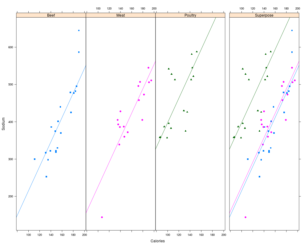
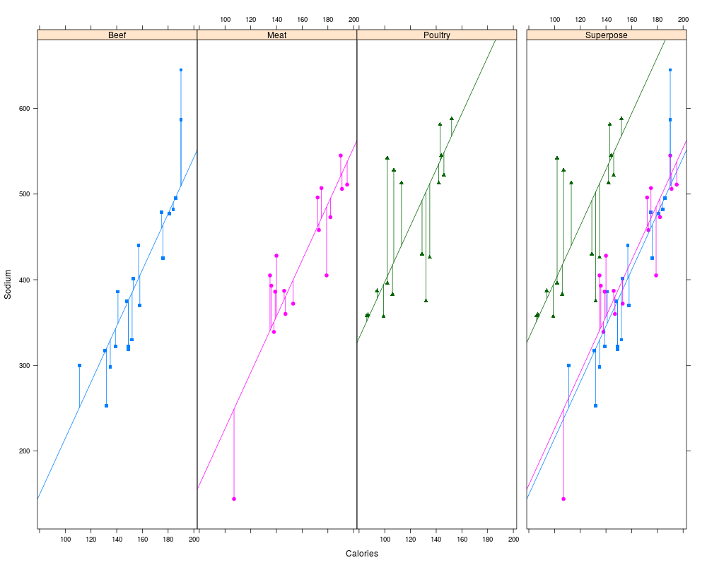
  ancovaplot(Sodium ~ Calories + Type, data=hotdog)
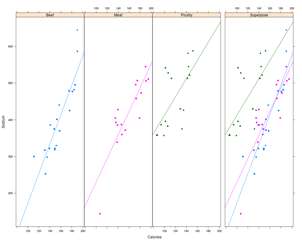
  ancovaplot(Sodium ~ Calories * Type, data=hotdog)
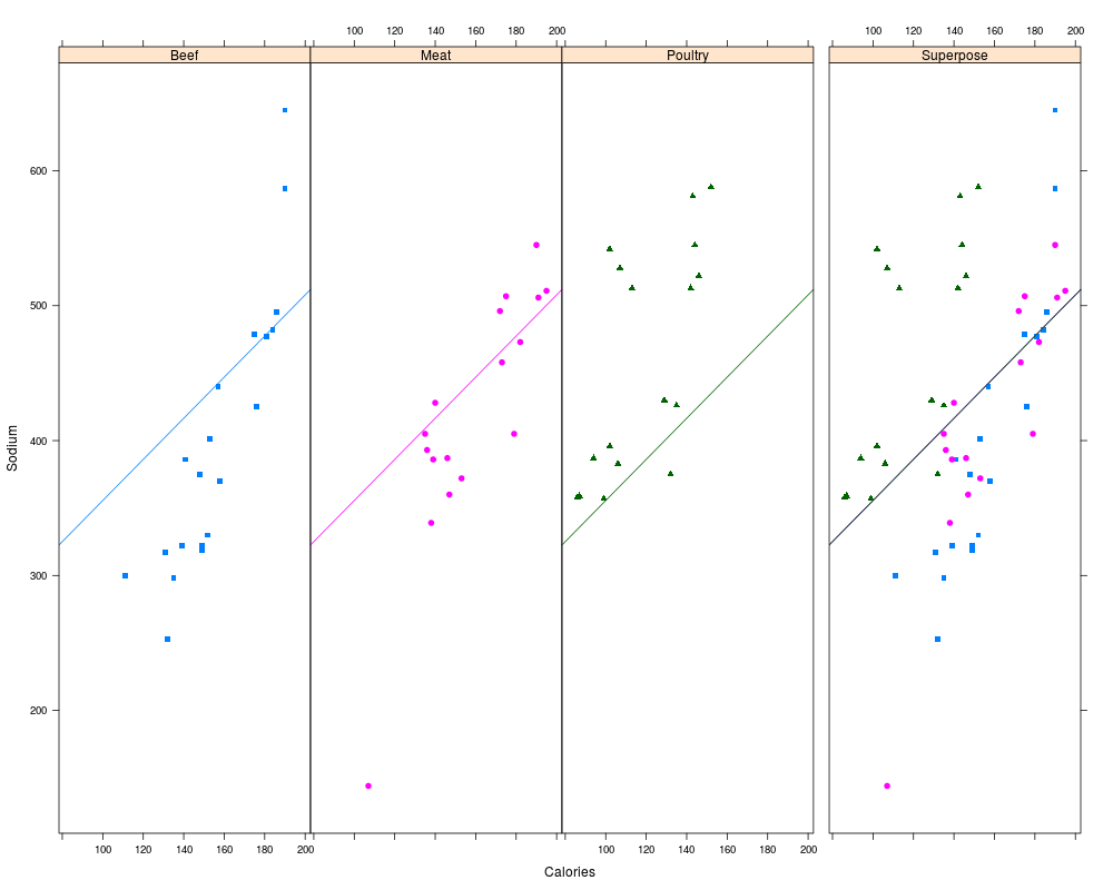
  ancovaplot(Sodium ~ Calories, groups=Type, data=hotdog)
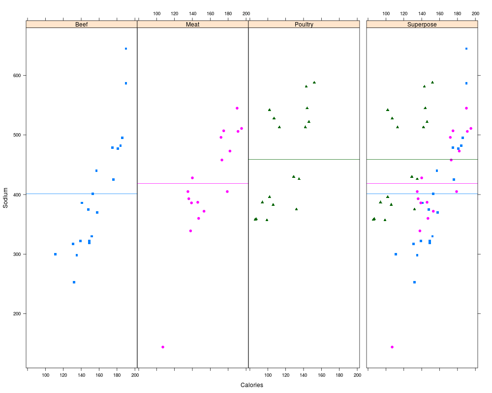
  ancovaplot(Sodium ~ Type, x=Calories, data=hotdog)

  ## Please see demo("ancova", package="HH") to coordinate placement
  ## of all four of these plots on the same page.

  ancovaplot(Sodium ~ Calories + Type, data=hotdog, plot.resids=TRUE)

Results


R version 3.3.1 (2016-06-21) -- "Bug in Your Hair"
Copyright (C) 2016 The R Foundation for Statistical Computing
Platform: x86_64-pc-linux-gnu (64-bit)

R is free software and comes with ABSOLUTELY NO WARRANTY.
You are welcome to redistribute it under certain conditions.
Type 'license()' or 'licence()' for distribution details.

R is a collaborative project with many contributors.
Type 'contributors()' for more information and
'citation()' on how to cite R or R packages in publications.

Type 'demo()' for some demos, 'help()' for on-line help, or
'help.start()' for an HTML browser interface to help.
Type 'q()' to quit R.

> library(HH)
Loading required package: lattice
Loading required package: grid
Loading required package: latticeExtra
Loading required package: RColorBrewer
Loading required package: multcomp
Loading required package: mvtnorm
Loading required package: survival
Loading required package: TH.data
Loading required package: MASS

Attaching package: 'TH.data'

The following object is masked from 'package:MASS':

    geyser

Loading required package: gridExtra
> png(filename="/home/ddbj/snapshot/RGM3/R_CC/result/HH/ancovaplot.Rd_%03d_medium.png", width=480, height=480)
> ### Name: ancovaplot
> ### Title: Analysis of Covariance Plots
> ### Aliases: ancovaplot ancovaplot.formula panel.ancova.superpose
> ### Keywords: hplot dplot models regression
> 
> ### ** Examples
> 
>   data(hotdog, package="HH")
>   ancovaplot(Sodium ~ Calories + Type, data=hotdog)
>   ancovaplot(Sodium ~ Calories * Type, data=hotdog)
>   ancovaplot(Sodium ~ Calories, groups=Type, data=hotdog)
>   ancovaplot(Sodium ~ Type, x=Calories, data=hotdog)
> 
>   ## Please see demo("ancova", package="HH") to coordinate placement
>   ## of all four of these plots on the same page.
> 
>   ancovaplot(Sodium ~ Calories + Type, data=hotdog, plot.resids=TRUE)
> 
> 
> 
> 
> 
> 
> dev.off()
null device 
          1 
>