For intxplot, a formula with a factor as the
predictor variable.
For panel.intxplot, standard argument for panel functions.
data
data.frame, as used in xyplot.
groups.in
groups.in, as used in xyplot.
scales
Optional, additional arguments for the standard scales
in xyplot.
key.length
Number of columns in the key.
key.lines
default value for the lines argument of key.
key
logical. If TRUE, draw the key.
trace.factor.name
Name of the grouping variable.
x.factor.name
name of the dependent variable.
xlab
as in xyplot, defaults to the name of the predictor variable
from the formula.
main
as in xyplot. Defaults to the main.title argument.
panel
as in xyplot. Defaults to the "panel.intxplot".
condition.name
name of the conditioning variable.
summary.function
The default sufficient finds the mean,
standard deviation, and sample size of the response variable for each
level of the conditioning factor. See sufficient.
se
standard errors to be passed to panel.intxplot.
se Missing, logical, or a numeric vector.
If missing or FALSE, standard errors are not plotted.
If se=TRUE in intxplot,
the standard errors are calculated from the
sufficient statistics for each group as the group's standard deviation
divided by the square root of the group's observation
count. If se is numeric vector, it is evaluated in the environment of
the sufficient statistics.
the se argument to panel.intxplot must be numeric.
,
...
In intxplot, arguments for panel.intxplot.
In panel.intxplot, arguments for panel.superpose.
data.is.summary
logical, defaults to FALSE under the
assumption that the input data.frame is the original data and the
intxplot function will generate the summary information
(primarily standard deviation sd and number of
observations nobs for each group). When TRUE, the
standard error calculation assumes variables sd and
nobs are in the dataset.
main.title
Default main title for plot.
main.cex
Default character expansion for main title.
y, subscripts, groups, type
Standard arguments for panel functions.
cv
critical value for confidence intervals. Defaults to 1.96.
offset.use
logical. If TRUE, offset the endpoints
of each group.
offset.scale
Scale number indicating how far apart the
ends of the groups will be placed. Larger numbers make them closer
together.
offset
Actual numbers by which the end of the groups are offset
from their nominal location which is the as.numeric of the
group levels.
rug.use
logical. If TRUE, display a rug for the endpoints
of each group.
Value
"trellis" object.
Author(s)
Richard M. Heiberger <rmh@temple.edu>
See Also
sufficient
Examples
## This uses the same data as the HH Section 12.13 rhizobium example.
data(rhiz.clover)
## interaction plot, no se
intxplot(Npg ~ strain, groups=comb, data=rhiz.clover)
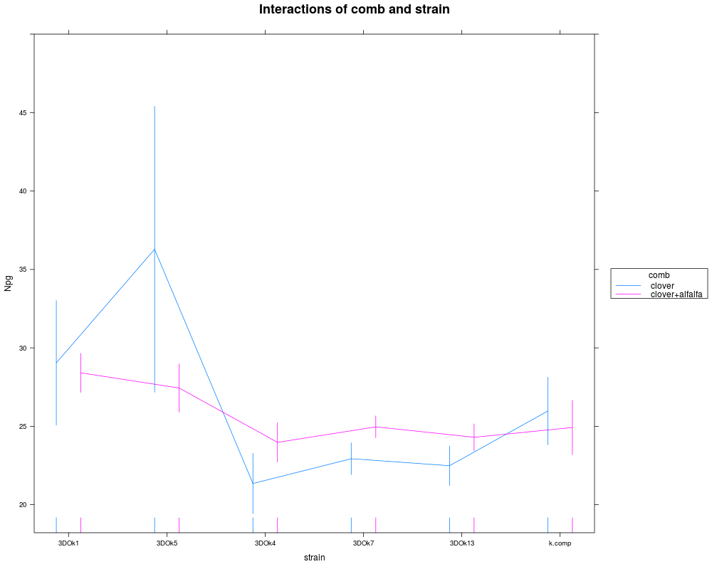
## interaction plot, individual se for each treatment combination
intxplot(Npg ~ strain, groups=comb, data=rhiz.clover, se=TRUE)
## Rescaled to allow the CI bars to stay within the plot region
intxplot(Npg ~ strain, groups=comb, data=rhiz.clover, se=TRUE,
ylim=range(rhiz.clover$Npg))
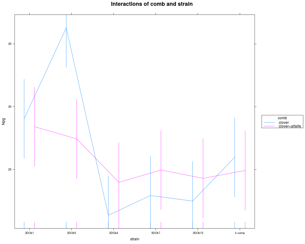
## interaction plot, common se based on ANOVA table
intxplot(Npg ~ strain, groups=comb, data=rhiz.clover,
se=sqrt(sum((nobs-1)*sd^2)/(sum(nobs-1)))/sqrt(5))
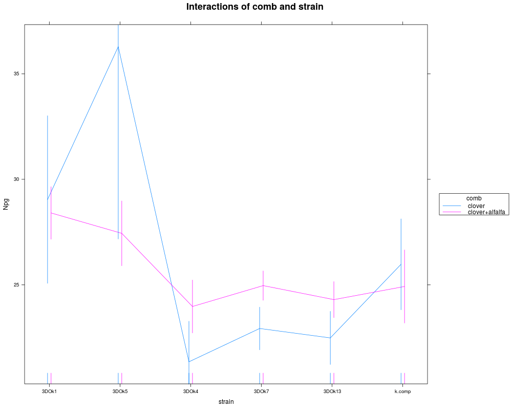
## Rescaled to allow the CI bars to stay within the plot region
intxplot(Npg ~ strain, groups=comb, data=rhiz.clover,
se=sqrt(sum((nobs-1)*sd^2)/(sum(nobs-1)))/sqrt(5),
ylim=range(rhiz.clover$Npg))
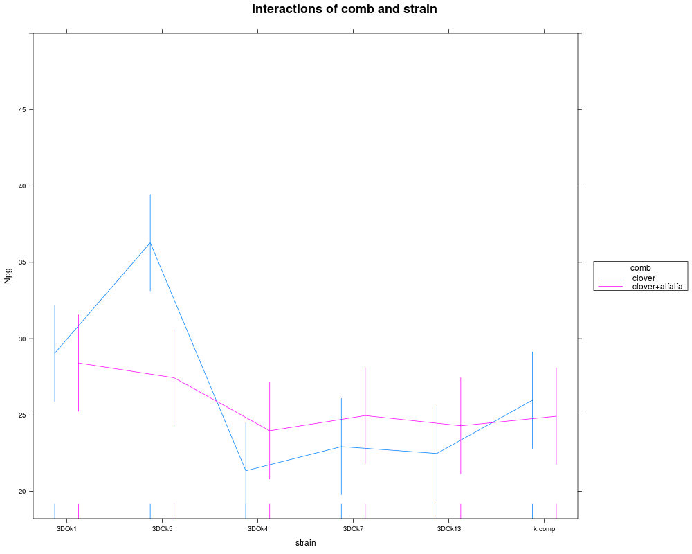
## change distance between endpoints
intxplot(Npg ~ strain, groups=comb, data=rhiz.clover,
se=TRUE, offset.scale=20)
## When data includes the nobs and sd variables, data.is.summary=TRUE is needed.
intxplot(Npg ~ strain, groups=comb,
se=sqrt(sum((nobs-1)*sd^2)/(sum(nobs-1)))/sqrt(5),
data=sufficient(rhiz.clover, y="Npg", c("strain","comb")),
data.is.summary=TRUE,
ylim=range(rhiz.clover$Npg))
Results
R version 3.3.1 (2016-06-21) -- "Bug in Your Hair"
Copyright (C) 2016 The R Foundation for Statistical Computing
Platform: x86_64-pc-linux-gnu (64-bit)

R is free software and comes with ABSOLUTELY NO WARRANTY.
You are welcome to redistribute it under certain conditions.
Type 'license()' or 'licence()' for distribution details.

R is a collaborative project with many contributors.
Type 'contributors()' for more information and
'citation()' on how to cite R or R packages in publications.

Type 'demo()' for some demos, 'help()' for on-line help, or
'help.start()' for an HTML browser interface to help.
Type 'q()' to quit R.

> library(HH)
Loading required package: lattice
Loading required package: grid
Loading required package: latticeExtra
Loading required package: RColorBrewer
Loading required package: multcomp
Loading required package: mvtnorm
Loading required package: survival
Loading required package: TH.data
Loading required package: MASS

Attaching package: 'TH.data'

The following object is masked from 'package:MASS':

    geyser

Loading required package: gridExtra
> png(filename="/home/ddbj/snapshot/RGM3/R_CC/result/HH/intxplot.Rd_%03d_medium.png", width=480, height=480)
> ### Name: intxplot
> ### Title: Interaction plot, with an option to print standard error bars.
> ### Aliases: intxplot panel.intxplot
> ### Keywords: dplot
>
> ### ** Examples
>
> ## This uses the same data as the HH Section 12.13 rhizobium example.
>
> data(rhiz.clover)
>
> ## interaction plot, no se
> intxplot(Npg ~ strain, groups=comb, data=rhiz.clover)
>
> ## interaction plot, individual se for each treatment combination
> intxplot(Npg ~ strain, groups=comb, data=rhiz.clover, se=TRUE)
>
> ## Rescaled to allow the CI bars to stay within the plot region
> intxplot(Npg ~ strain, groups=comb, data=rhiz.clover, se=TRUE,
+          ylim=range(rhiz.clover$Npg))
>
> ## interaction plot, common se based on ANOVA table
> intxplot(Npg ~ strain, groups=comb, data=rhiz.clover,
+          se=sqrt(sum((nobs-1)*sd^2)/(sum(nobs-1)))/sqrt(5))
>
> ## Rescaled to allow the CI bars to stay within the plot region
> intxplot(Npg ~ strain, groups=comb, data=rhiz.clover,
+          se=sqrt(sum((nobs-1)*sd^2)/(sum(nobs-1)))/sqrt(5),
+          ylim=range(rhiz.clover$Npg))
>
> ## change distance between endpoints
> intxplot(Npg ~ strain, groups=comb, data=rhiz.clover,
+          se=TRUE, offset.scale=20)
>
> ## When data includes the nobs and sd variables, data.is.summary=TRUE is needed.
> intxplot(Npg ~ strain, groups=comb,
+          se=sqrt(sum((nobs-1)*sd^2)/(sum(nobs-1)))/sqrt(5),
+          data=sufficient(rhiz.clover, y="Npg", c("strain","comb")),
+          data.is.summary=TRUE,
+          ylim=range(rhiz.clover$Npg))
>
>
>
>
>
> dev.off()
null device
          1
>
 .
.