Supported by Dr. Osamu Ogasawara and  . . |
|
Last data update: 2014.03.03 |
Diverging stacked barcharts for Likert, semantic differential, rating scale data, and population pyramids.DescriptionConstructs and plots diverging stacked barcharts for Likert, semantic differential, rating scale data, and population pyramids. Usage
likert(x, ...)
likertplot(x, ...)
## S3 method for class 'likert'
plot(x, ...)

## S3 method for class 'formula'
plot.likert(x, data, ReferenceZero=NULL, value, levelsName="",
            scales.in=NULL,   ## use scales=
            between=list(x=1 + (horizontal), y=.5 + 2*(!horizontal)),
            auto.key.in=NULL, ## use auto.key=
            panel.in=NULL,    ## use panel=
            horizontal=TRUE,
            par.settings.in=NULL, ## use par.settings=
            ...,
            as.percent = FALSE,
            ## titles
            ylab= if (horizontal) {
              if (length(x)==3)
                deparse(x[[2]])
              else
                "Question"
            }
            else
            if (as.percent != FALSE) "Percent" else "Count",
            xlab= if (!horizontal) {
              if (length(x)==3)
                deparse(x[[2]])
              else
                "Question"
            }
            else
            if (as.percent != FALSE) "Percent" else "Count",
            main = x.sys.call,
            ## right axis
            rightAxisLabels = rowSums(data.list$Nums),
            rightAxis = !missing(rightAxisLabels),
            ylab.right = if (rightAxis) "Row Count Totals" else NULL,
            xlab.top = NULL,
            right.text.cex =
              if (horizontal) { ## lazy evaluation
                if (!is.null(scales$y$cex)) scales$y$cex else .8
              }
              else
                {
                  if (!is.null(scales$x$cex)) scales$x$cex else .8
                },

            ## scales
            xscale.components = xscale.components.top.HH,
            yscale.components = yscale.components.right.HH,
            xlimEqualLeftRight = FALSE,
            xTickLabelsPositive = TRUE,
            ## row sequencing
            as.table=TRUE,
            positive.order=FALSE,
            data.order=FALSE,
            reverse=ifelse(horizontal, as.table, FALSE),
            ## resizePanels arguments
            h.resizePanels=sapply(result$y.used.at, length),
            w.resizePanels=sapply(result$x.used.at, length),
            ## color options
            reference.line.col="gray65",
            key.border.white=TRUE,
            col=likertColor(Nums.attr$nlevels,
              ReferenceZero=ReferenceZero,
              colorFunction=colorFunction,
              colorFunctionOption=colorFunctionOption),
            colorFunction="diverge_hcl",
            colorFunctionOption="lighter"
            )
## Default S3 method:
plot.likert(x,
            positive.order=FALSE,
            ylab=names(dimnames(x)[1]),
            xlab=if (as.percent != FALSE) "Percent" else "Count",
            main=xName,
            reference.line.col="gray65",
            col.strip.background="gray97",
            col=likertColor(attr(x, "nlevels"),
              ReferenceZero=ReferenceZero,
              colorFunction=colorFunction,
              colorFunctionOption=colorFunctionOption),
            colorFunction="diverge_hcl",
            colorFunctionOption="lighter",
            as.percent=FALSE,
            par.settings.in=NULL,
            horizontal=TRUE,
            ReferenceZero=NULL,
            ...,
            key.border.white=TRUE,
            xName=deparse(substitute(x)),
            rightAxisLabels=rowSums(abs(x)),
            rightAxis=!missing(rightAxisLabels),
            ylab.right=if (rightAxis) "Row Count Totals" else NULL,
            panel=panel.barchart,
            xscale.components=xscale.components.top.HH,
            yscale.components=yscale.components.right.HH,
            xlimEqualLeftRight=FALSE,
            xTickLabelsPositive=TRUE,
            reverse=FALSE)

## S3 method for class 'array'
plot.likert(x,
             condlevelsName=paste("names(dimnames(", xName, "))[-(1:2)]",
                                  sep=""),
             xName=deparse(substitute(x)),
             main=paste("layers of", xName, "by", condlevelsName),
             ...)

## S3 method for class 'likert'
plot.likert(x, ...)  ## See Details

## S3 method for class 'list'
plot.likert(x,  ## named list of matrices, 2D tables,
                               ## 2D ftables, or 2D structables,
                               ## or all-numeric data.frames
            condlevelsName="ListNames",
            xName=deparse(substitute(x)),
            main=paste("List items of", xName, "by", condlevelsName),
            layout=if (length(dim.x) > 1) dim.x else {
                               if (horizontal) c(1, length(x)) else c(length(x), 1)},
            positive.order=FALSE,
            strip=!horizontal,
            strip.left=horizontal,
            strip.left.values=names(x),
            strip.values=names(x),
            strip.par=list(cex=1, lines=1),
            strip.left.par=list(cex=1, lines=1),
            horizontal=TRUE,
            ...,
            rightAxisLabels=sapply(x, function(x) rowSums(abs(x)), simplify = FALSE),
            rightAxis=!missing(rightAxisLabels),
            resize.height.tuning=-.5,
            resize.height=if (missing(layout) || length(dim.x) != 2) {
              c("nrow","rowSums")
            } else {
              rep(1, layout[2])
            },
            resize.width=if (missing(layout)) {1 } else {
              rep(1, layout[1])
            },
            box.ratio=if (
              length(resize.height)==1 &&
              resize.height == "rowSums") 1000 else 2,
            xscale.components=xscale.components.top.HH,
            yscale.components=yscale.components.right.HH)

## S3 method for class 'table'
plot.likert(x, ..., xName=deparse(substitute(x)))
## S3 method for class 'ftable'
plot.likert(x, ..., xName=deparse(substitute(x)))
## S3 method for class 'structable'
plot.likert(x, ..., xName=deparse(substitute(x)))

## S3 method for class 'data.frame'
plot.likert(x, ..., xName=deparse(substitute(x)))


xscale.components.top.HH(...)
yscale.components.right.HH(...)
Arguments
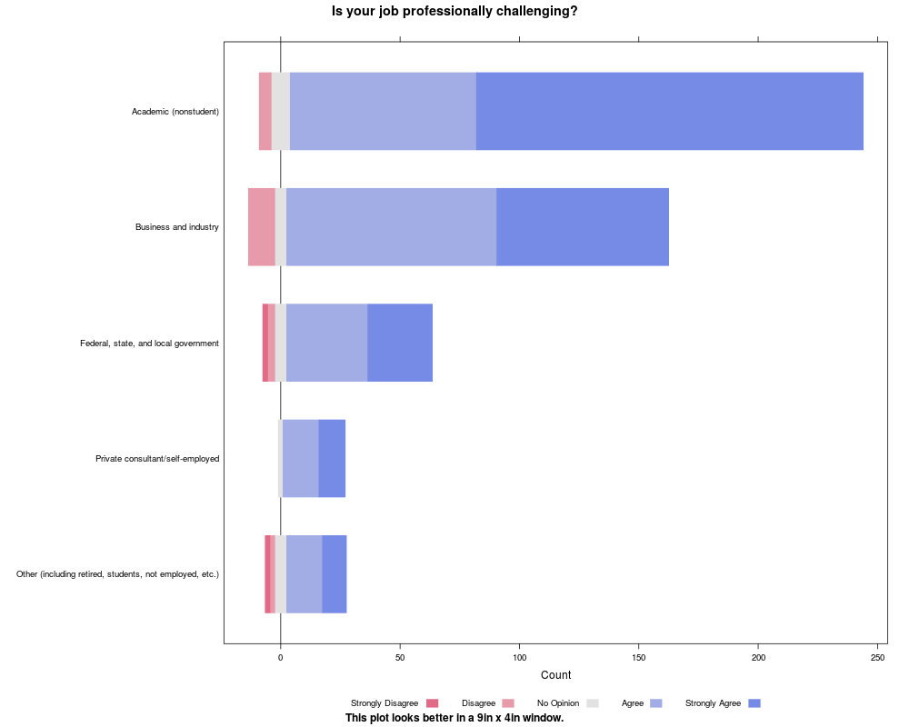
DetailsThe counts (or percentages) of respondents on each row who agree with
the statement are shown to the right of the zero line; the counts (or
percentages) who disagree are shown to the left. The counts (or
percentages) for respondents who neither agree nor disagree are split
down the middle and are shown in a neutral color. The neutral category
is omitted when the scale has an even number of choices.
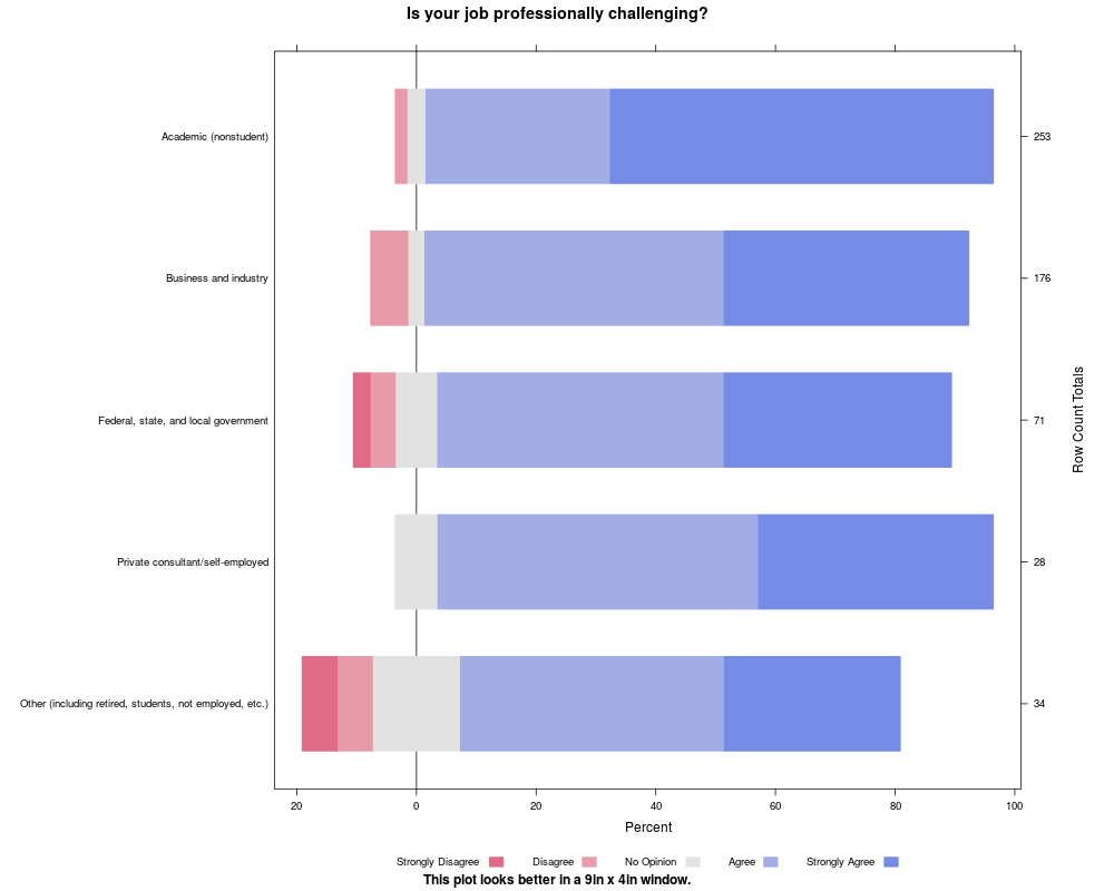
It is difficult to compare
lengths without a common baseline. In this situation, we are primarily
interested in the total count (or percent) to the right or left of the
zero line; the breakdown into strongly or not is of lesser interest so
that the primary comparisons do have a common baseline of zero. The
rows within each panel are displayed in their original order by
default. If the argument Diverging stacked barcharts are also called "two-directional stacked barcharts". Some authors use the term "floating barcharts" for vertical diverging stacked barcharts and the term "sliding barcharts" for horizontal diverging stacked barcharts. All items in a list of named two-dimensional objects must have the
same number of columns. If the items have different column names, the
column names of the last item in the list will be used in the key. If
the dimnames of the matrices are named, the names will be used in the
plot. It is possible to produce a likert plot with a list of objects
with different numbers of columns, but not with the
A single data.frame
The ValueA NoteThe current version of the
NoteAnn Liu-Ferrara was a beta tester for the shiny app. Note
Author(s)Richard M. Heiberger, with contributions from Naomi B. Robbins <naomi@nbr-graphs.com>. Maintainer: Richard M. Heiberger <rmh@temple.edu> ReferencesRichard M. Heiberger, Naomi B. Robbins (2014)., "Design of Diverging Stacked Bar Charts for Likert Scales and Other Applications", Journal of Statistical Software, 57(5), 1–32, http://www.jstatsoft.org/v57/i05/. Richard Heiberger and Naomi Robbins (2011), "Alternative to Charles Blow's Figure in "Newt's War on Poor Children"", Forbes OnLine, December 20, 2011. http://www.forbes.com/sites/naomirobbins/2011/12/20/alternative-to-charles-blows-figure-in-newts-war-on-poor-children-2/ Naomi Robbins (2011), "Visualizing Data: Challenges to Presentation of Quality Graphics—and Solutions", Amstat News, September 2011, 28–30. http://magazine.amstat.org/blog/2011/09/01/visualizingdata/ Naomi B. Robbins and Richard M. Heiberger (2011). Plotting Likert and
Other Rating Scales. In JSM Proceedings, Section on Survey Research
Methods. Alexandria, VA: American Statistical Association, 1058–1066. Luo, Amy and Tim Keyes (2005). "Second Set of Results in from the Career Track Member Survey," Amstat News. Arlington, VA: American Statistical Association. See Also
Examples
## See file HH/demo/likert-paper.r for a complete set of examples using
## the formula method into the underlying lattice:::barchart plotting
## technology. See file HH/demo/likert-paper-noFormula.r for the same
## set of examples using the matrix and list of matrices methods. See
## file HH/demo/likertMosaic-paper.r for the same set of examples using
## the still experimental functions built on the vcd:::mosaic as the
## underlying plotting technology
data(ProfChal) ## ProfChal is a data.frame.
## See below for discussion of the dataset.
## Count plot
likert(Question ~ . , ProfChal[ProfChal$Subtable=="Employment sector",],
main='Is your job professionally challenging?',
ylab=NULL,
sub="This plot looks better in a 9in x 4in window.")
## Percent plot calculated automatically from Count data
likert(Question ~ . , ProfChal[ProfChal$Subtable=="Employment sector",],
as.percent=TRUE,
main='Is your job professionally challenging?',
ylab=NULL,
sub="This plot looks better in a 9in x 4in window.")
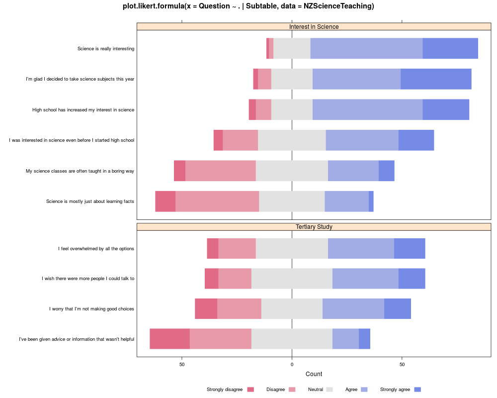
## formula method
data(NZScienceTeaching)
likert(Question ~ . | Subtable, data=NZScienceTeaching,
ylab=NULL,
scales=list(y=list(relation="free")), layout=c(1,2))
## Not run:
## formula notation with expanded right-hand-side
likert(Question ~
"Strongly disagree" + Disagree + Neutral + Agree + "Strongly agree" |
Subtable, data=NZScienceTeaching,
ylab=NULL,
scales=list(y=list(relation="free")), layout=c(1,2))
## End(Not run)
## Not run:
## formula notation with long data arrangement
NZScienceTeachingLong <- reshape2::melt(NZScienceTeaching,
id.vars=c("Question", "Subtable"))
names(NZScienceTeachingLong)[3] <- "Agreement"
head(NZScienceTeachingLong)
likert(Question ~ Agreement | Subtable, value="value", data=NZScienceTeachingLong,
ylab=NULL,
scales=list(y=list(relation="free")), layout=c(1,2))
## End(Not run)
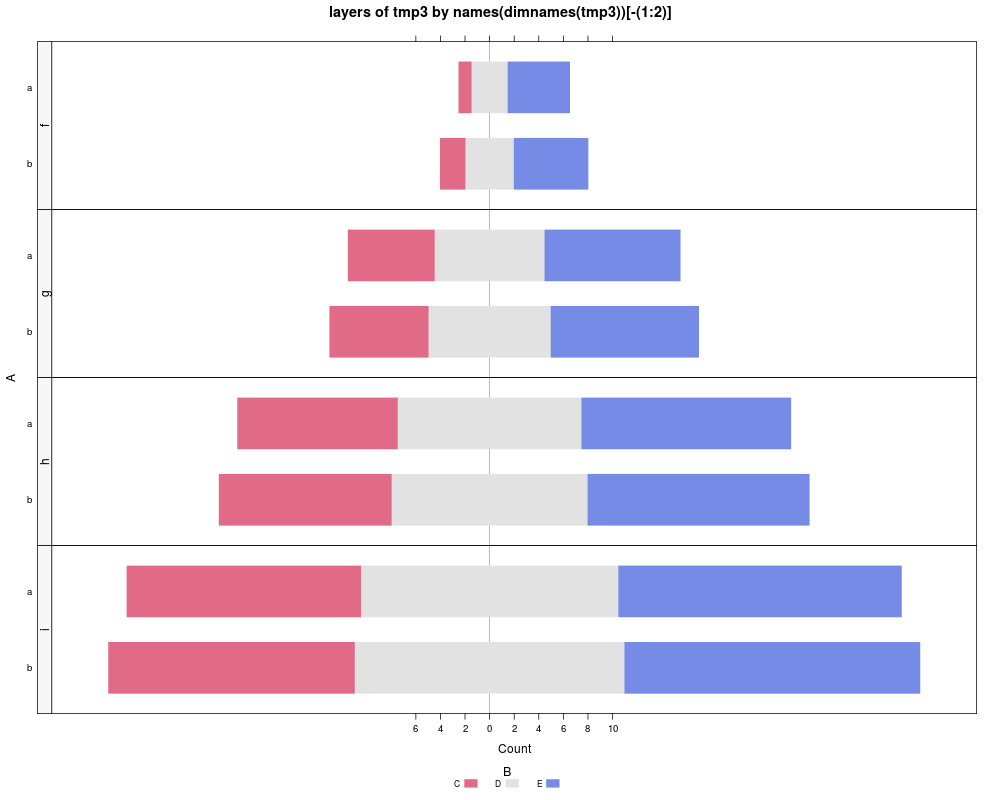
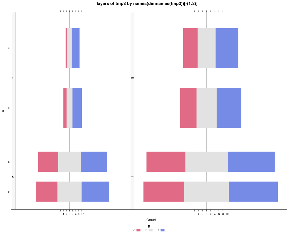
## Examples with higher-dimensional arrays.
tmp3 <- array(1:24, dim=c(2,3,4),
dimnames=list(A=letters[1:2], B=LETTERS[3:5], C=letters[6:9]))
## positive.order=FALSE is the default. With arrays
## the rownames within each item of an array are identical.
## likert(tmp3)
likert(tmp3, layout=c(1,4))
likert(tmp3, layout=c(2,2), resize.height=c(2,1), resize.width=c(3,4))
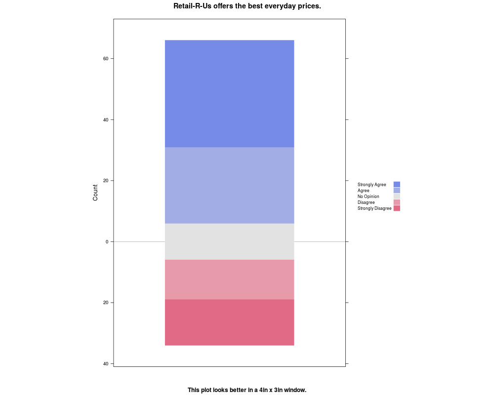
## plot.likert interprets vectors as single-row matrices.
## http://survey.cvent.com/blog/customer-insights-2/box-scores-are-not-just-for-baseball
Responses <- c(15, 13, 12, 25, 35)
names(Responses) <- c("Strongly Disagree", "Disagree", "No Opinion",
"Agree", "Strongly Agree")
## Not run:
likert(Responses, main="Retail-R-Us offers the best everyday prices.",
sub="This plot looks better in a 9in x 2.6in window.")
## End(Not run)
## reverse=TRUE is needed for a single-column key with
## horizontal=FALSE and with space="right"
likert(Responses, horizontal=FALSE,
aspect=1.5,
main="Retail-R-Us offers the best everyday prices.",
auto.key=list(space="right", columns=1,
reverse=TRUE, padding.text=2),
sub="This plot looks better in a 4in x 3in window.")
## Not run:
## Since age is always positive and increases in a single direction,
## this example uses colors from a sequential palette for the age
## groups. In this example we do not use a diverging palette that is
## appropriate when groups are defined by a characteristic, such as
## strength of agreement or disagreement, that can increase in two directions.
## Initially we use the default Blue palette in the sequential_hcl function.
likert(AudiencePercent,
auto.key=list(between=1, between.columns=2),
xlab=paste("Percentage of audience younger than 35 (left of zero)",
"and older than 35 (right of zero)"),
main="Target Audience",
col=rev(sequential_hcl(4)),
sub="This plot looks better in a 7in x 3.5in window.")
## The really light colors in the previous example are too light.
## Therefore we use the col argument directly. We chose to use an
## intermediate set of Blue colors selected from a longer Blue palette.
likert(AudiencePercent,
positive.order=TRUE,
auto.key=list(between=1, between.columns=2),
xlab=paste("Percentage of audience younger than 35",
"(left of zero) and older than 35 (right of zero)"),
main="Brand A has the most even distribution of ages",
col=sequential_hcl(11)[5:2],
scales=list(x=list(at=seq(-90,60,10),
labels=as.vector(rbind("",seq(-80,60,20))))),
sub="This plot looks better in a 7in x 3.5in window.")
## End(Not run)
## Not run:
## See the ?as.pyramidLikert help page for these examples
## Population Pyramid
data(USAge.table)
USA79 <- USAge.table[75:1, 2:1, "1979"]/1000000
PL <- likert(USA79,
main="Population of United States 1979 (ages 0-74)",
xlab="Count in Millions",
ylab="Age",
scales=list(
y=list(
limits=c(0,77),
at=seq(1,76,5),
labels=seq(0,75,5),
tck=.5))
)
PL
as.pyramidLikert(PL)
likert(USAge.table[75:1, 2:1, c("1939","1959","1979")]/1000000,
main="Population of United States 1939,1959,1979 (ages 0-74)",
sub="Look for the Baby Boom",
xlab="Count in Millions",
ylab="Age",
scales=list(
y=list(
limits=c(0,77),
at=seq(1,76,5),
labels=seq(0,75,5),
tck=.5)),
strip.left=FALSE, strip=TRUE,
layout=c(3,1), between=list(x=.5))
## End(Not run)
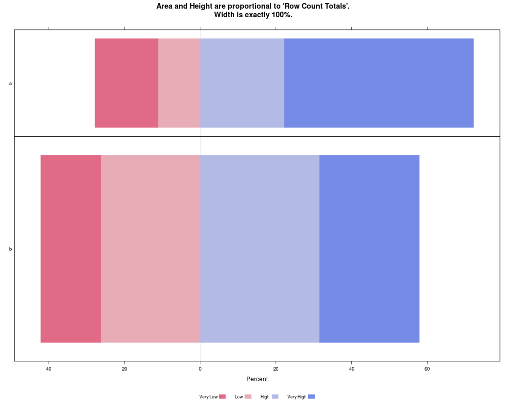
Pop <- rbind(a=c(3,2,4,9), b=c(6,10,12,10))
dimnames(Pop)[[2]] <- c("Very Low", "Low", "High", "Very High")
likert(as.listOfNamedMatrices(Pop),
as.percent=TRUE,
resize.height="rowSums",
strip=FALSE,
strip.left=FALSE,
main=paste("Area and Height are proportional to 'Row Count Totals'.",
"Width is exactly 100%.", sep="\n"))
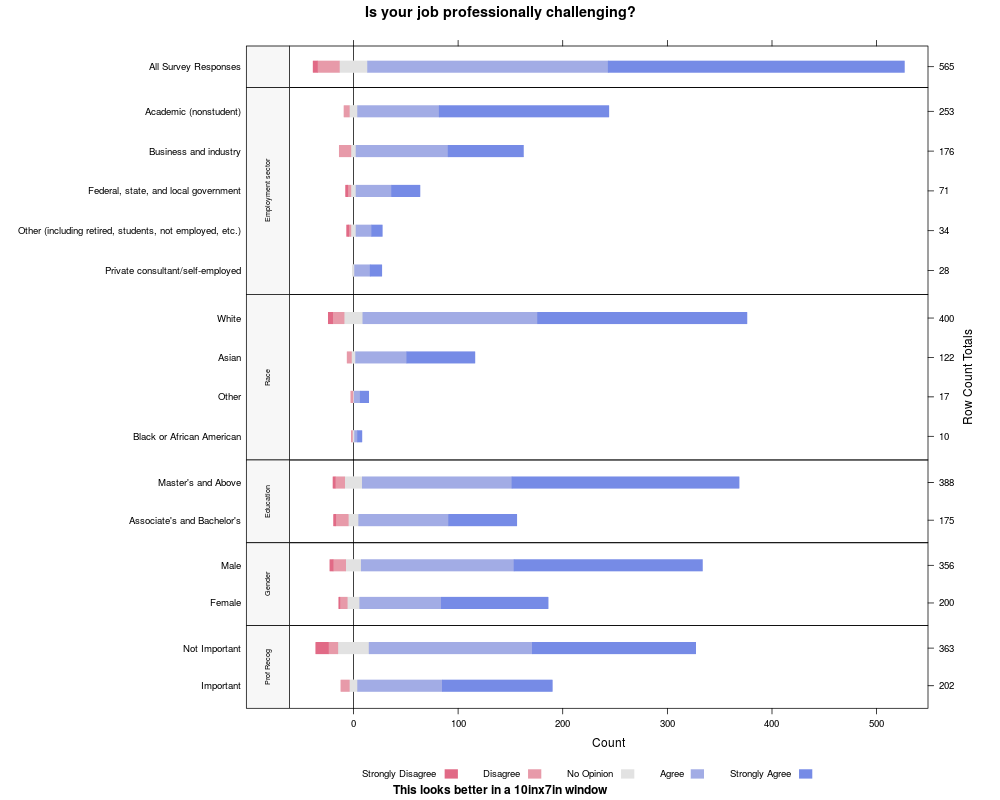
## Professional Challenges example.
##
## The data for this example is a list of related likert scales, with
## each item in the list consisting of differently named rows. The data
## is from a questionnaire analyzed in a recent Amstat News article.
## The study population was partitioned in several ways. Data from one
## of the partitions (Employment sector) was used in the first example
## in this help file. The examples here show various options for
## displaying all partitions on the same plot.
##
data(ProfChal)
levels(ProfChal$Subtable)[6] <- "Prof Recog" ## reduce length of label
## 1. Plot counts with rows in each panel sorted by positive counts.
##
## Not run:
likert(Question ~ . | Subtable, ProfChal,
positive.order=TRUE,
main="This works, but needs more specified arguments to look good")
likert(Question ~ . | Subtable, ProfChal,
scales=list(y=list(relation="free")), layout=c(1,6),
positive.order=TRUE,
between=list(y=0),
strip=FALSE, strip.left=strip.custom(bg="gray97"),
par.strip.text=list(cex=.6, lines=5),
main="Is your job professionally challenging?",
ylab=NULL,
sub="This looks better in a 10inx7in window")
## End(Not run)
ProfChalCountsPlot <-
likert(Question ~ . | Subtable, ProfChal,
scales=list(y=list(relation="free")), layout=c(1,6),
positive.order=TRUE,
box.width=unit(.4,"cm"),
between=list(y=0),
strip=FALSE, strip.left=strip.custom(bg="gray97"),
par.strip.text=list(cex=.6, lines=5),
main="Is your job professionally challenging?",
rightAxis=TRUE, ## display Row Count Totals
ylab=NULL,
sub="This looks better in a 10inx7in window")
ProfChalCountsPlot
## Not run:
## 2. Plot percents with rows in each panel sorted by positive percents.
## This is a different sequence than the counts. Row Count Totals are
## displayed on the right axis.
ProfChalPctPlot <-
likert(Question ~ . | Subtable, ProfChal,
as.percent=TRUE, ## implies display Row Count Totals
scales=list(y=list(relation="free")), layout=c(1,6),
positive.order=TRUE,
box.width=unit(.4,"cm"),
between=list(y=0),
strip=FALSE, strip.left=strip.custom(bg="gray97"),
par.strip.text=list(cex=.6, lines=5),
main="Is your job professionally challenging?",
rightAxis=TRUE, ## display Row Count Totals
ylab=NULL,
sub="This looks better in a 10inx7in window")
ProfChalPctPlot
## 3. Putting both percents and counts on the same plot, both in
## the order of the positive percents.
LikertPercentCountColumns(Question ~ . | Subtable, ProfChal,
layout=c(1,6), scales=list(y=list(relation="free")),
ylab=NULL, between=list(y=0),
strip.left=strip.custom(bg="gray97"), strip=FALSE,
par.strip.text=list(cex=.7),
positive.order=TRUE,
main="Is your job professionally challenging?")
## Restore original name
## levels(ProfChal$Subtable)[6] <- "Attitude\ntoward\nProfessional\nRecognition"
## End(Not run)
## Not run:
## 4. All possible forms of formula for the likert formula method:
data(ProfChal)
row.names(ProfChal) <- abbreviate(ProfChal$Question, 8)
likert( Question ~ . | Subtable,
data=ProfChal, scales=list(y=list(relation="free")), layout=c(1,6))
likert( Question ~
"Strongly Disagree" + Disagree + "No Opinion" + Agree + "Strongly Agree" | Subtable,
data=ProfChal, scales=list(y=list(relation="free")), layout=c(1,6))
likert( Question ~ . ,
data=ProfChal)
likert( Question ~ "Strongly Disagree" + Disagree + "No Opinion" + Agree + "Strongly Agree",
data=ProfChal)
likert( ~ . | Subtable,
data=ProfChal, scales=list(y=list(relation="free")), layout=c(1,6))
likert( ~ "Strongly Disagree" + Disagree + "No Opinion" + Agree + "Strongly Agree" | Subtable,
data=ProfChal, scales=list(y=list(relation="free")), layout=c(1,6))
likert( ~ . ,
data=ProfChal)
likert( ~ "Strongly Disagree" + Disagree + "No Opinion" + Agree + "Strongly Agree",
data=ProfChal)
## End(Not run)
## Not run:
## 5. putting the x-axis tick labels on top for horizontal plots
## putting the y-axis tick lables on right for vertical plots
##
## This non-standard specification is a consequence of using the right
## axis labels for different values than appear on the left axis labels
## with horizontal plots, and using the top axis labels for different
## values than appear on the bottom axis labels with vertical plots.
## Percent plot calculated automatically from Count data
tmph <-
likert(Question ~ . , ProfChal[ProfChal$Subtable=="Employment sector",],
as.percent=TRUE,
main='Is your job professionally challenging?',
ylab=NULL,
sub="This plot looks better in a 9in x 4in window.")
tmph$x.scales$labels
names(tmph$x.scales$labels) <- tmph$x.scales$labels
update(tmph, scales=list(x=list(alternating=2)), xlab=NULL, xlab.top="Percent")
tmpv <-
likert(Question ~ . , ProfChal[ProfChal$Subtable=="Employment sector",],
as.percent=TRUE,
main='Is your job professionally challenging?',
sub="likert plots with long Question names look better horizontally.
With effort they can be made to look adequate vertically.",
horizontal=FALSE,
scales=list(y=list(alternating=2), x=list(rot=c(90, 0))),
ylab.right="Percent",
ylab=NULL,
xlab.top="Column Count Totals",
par.settings=list(
layout.heights=list(key.axis.padding=5),
layout.widths=list(key.right=1.5, right.padding=0))
)
tmpv$y.scales$labels
names(tmpv$y.scales$labels) <- tmpv$y.scales$labels
tmpv
tmpv$x.limits <- abbreviate(tmpv$x.limits,8)
tmpv$x.scales$rot=c(0, 0)
tmpv
## End(Not run)
## Not run:
## run the shiny app
shiny::runApp(system.file("shiny/likert", package="HH"))
## End(Not run)
## The ProfChal data is done again with explicit use of ResizeEtc
## in ?HH:::ResizeEtc
Results
R version 3.3.1 (2016-06-21) -- "Bug in Your Hair"
Copyright (C) 2016 The R Foundation for Statistical Computing
Platform: x86_64-pc-linux-gnu (64-bit)

R is free software and comes with ABSOLUTELY NO WARRANTY.
You are welcome to redistribute it under certain conditions.
Type 'license()' or 'licence()' for distribution details.

R is a collaborative project with many contributors.
Type 'contributors()' for more information and
'citation()' on how to cite R or R packages in publications.

Type 'demo()' for some demos, 'help()' for on-line help, or
'help.start()' for an HTML browser interface to help.
Type 'q()' to quit R.

> library(HH)
Loading required package: lattice
Loading required package: grid
Loading required package: latticeExtra
Loading required package: RColorBrewer
Loading required package: multcomp
Loading required package: mvtnorm
Loading required package: survival
Loading required package: TH.data
Loading required package: MASS

Attaching package: 'TH.data'

The following object is masked from 'package:MASS':

    geyser

Loading required package: gridExtra
> png(filename="/home/ddbj/snapshot/RGM3/R_CC/result/HH/likert.Rd_%03d_medium.png", width=480, height=480)
> ### Name: likert
> ### Title: Diverging stacked barcharts for Likert, semantic differential,
> ###   rating scale data, and population pyramids.
> ### Aliases: likert plot.likert likertplot plot.likert.formula
> ###   plot.likert.default plot.likert.array plot.likert.likert
> ###   plot.likert.list plot.likert.table plot.likert.ftable
> ###   plot.likert.structable plot.likert.data.frame
> ###   xscale.components.top.HH yscale.components.right.HH floating pyramid
> ###   sliding semantic differential
> ### Keywords: hplot
>
> ### ** Examples
>
>
> ## See file HH/demo/likert-paper.r for a complete set of examples using
> ## the formula method into the underlying lattice:::barchart plotting
> ## technology.  See file HH/demo/likert-paper-noFormula.r for the same
> ## set of examples using the matrix and list of matrices methods.  See
> ## file HH/demo/likertMosaic-paper.r for the same set of examples using
> ## the still experimental functions built on the vcd:::mosaic as the
> ## underlying plotting technology
>
> data(ProfChal)  ## ProfChal is a data.frame.
> ## See below for discussion of the dataset.
>
>
> ## Count plot
> likert(Question ~ . , ProfChal[ProfChal$Subtable=="Employment sector",],
+        main='Is your job professionally challenging?',
+        ylab=NULL,
+        sub="This plot looks better in a 9in x 4in window.")
>
> ## Percent plot calculated automatically from Count data
> likert(Question ~ . , ProfChal[ProfChal$Subtable=="Employment sector",],
+        as.percent=TRUE,
+        main='Is your job professionally challenging?',
+        ylab=NULL,
+        sub="This plot looks better in a 9in x 4in window.")
>
> ## formula method
> data(NZScienceTeaching)
> likert(Question ~ . | Subtable, data=NZScienceTeaching,
+        ylab=NULL,
+        scales=list(y=list(relation="free")), layout=c(1,2))
>
> ## Not run:
> ##D ## formula notation with expanded right-hand-side
> ##D likert(Question ~
> ##D        "Strongly disagree" + Disagree + Neutral + Agree + "Strongly agree" |
> ##D        Subtable, data=NZScienceTeaching,
> ##D        ylab=NULL,
> ##D        scales=list(y=list(relation="free")), layout=c(1,2))
> ## End(Not run)
>
> ## Not run:
> ##D ## formula notation with long data arrangement
> ##D NZScienceTeachingLong <- reshape2::melt(NZScienceTeaching,
> ##D                                         id.vars=c("Question", "Subtable"))
> ##D names(NZScienceTeachingLong)[3] <- "Agreement"
> ##D head(NZScienceTeachingLong)
> ##D
> ##D likert(Question ~ Agreement | Subtable, value="value", data=NZScienceTeachingLong,
> ##D        ylab=NULL,
> ##D        scales=list(y=list(relation="free")), layout=c(1,2))
> ## End(Not run)
>
> ## Examples with higher-dimensional arrays.
> tmp3 <- array(1:24, dim=c(2,3,4),
+               dimnames=list(A=letters[1:2], B=LETTERS[3:5], C=letters[6:9]))
>
> ## positive.order=FALSE is the default.  With arrays
> ## the rownames within each item of an array are identical.
>
> ## likert(tmp3)
> likert(tmp3, layout=c(1,4))
> likert(tmp3, layout=c(2,2), resize.height=c(2,1), resize.width=c(3,4))
>
>
> ## plot.likert interprets vectors as single-row matrices.
> ## http://survey.cvent.com/blog/customer-insights-2/box-scores-are-not-just-for-baseball
> Responses <- c(15, 13, 12, 25, 35)
> names(Responses) <- c("Strongly Disagree", "Disagree", "No Opinion",
+                       "Agree", "Strongly Agree")
> ## Not run:
> ##D likert(Responses, main="Retail-R-Us offers the best everyday prices.",
> ##D        sub="This plot looks better in a 9in x 2.6in window.")
> ## End(Not run)
> ## reverse=TRUE  is needed for a single-column key with
> ## horizontal=FALSE and with space="right"
> likert(Responses, horizontal=FALSE,
+        aspect=1.5,
+        main="Retail-R-Us offers the best everyday prices.",
+        auto.key=list(space="right", columns=1,
+                      reverse=TRUE, padding.text=2),
+        sub="This plot looks better in a 4in x 3in window.")
>
>
> ## Not run:
> ##D ## Since age is always positive and increases in a single direction,
> ##D ## this example uses colors from a sequential palette for the age
> ##D ## groups.  In this example we do not use a diverging palette that is
> ##D ## appropriate when groups are defined by a characteristic, such as
> ##D ## strength of agreement or disagreement, that can increase in two directions.
> ##D
> ##D ## Initially we use the default Blue palette in the sequential_hcl function.
> ##D likert(AudiencePercent,
> ##D        auto.key=list(between=1, between.columns=2),
> ##D        xlab=paste("Percentage of audience younger than 35 (left of zero)",
> ##D                   "and older than 35 (right of zero)"),
> ##D        main="Target Audience",
> ##D        col=rev(sequential_hcl(4)),
> ##D        sub="This plot looks better in a 7in x 3.5in window.")
> ##D
> ##D ## The really light colors in the previous example are too light.
> ##D ## Therefore we use the col argument directly.  We chose to use an
> ##D ## intermediate set of Blue colors selected from a longer Blue palette.
> ##D likert(AudiencePercent,
> ##D        positive.order=TRUE,
> ##D        auto.key=list(between=1, between.columns=2),
> ##D        xlab=paste("Percentage of audience younger than 35",
> ##D          "(left of zero) and older than 35 (right of zero)"),
> ##D        main="Brand A has the most even distribution of ages",
> ##D        col=sequential_hcl(11)[5:2],
> ##D        scales=list(x=list(at=seq(-90,60,10),
> ##D                      labels=as.vector(rbind("",seq(-80,60,20))))),
> ##D       sub="This plot looks better in a 7in x 3.5in window.")
> ## End(Not run)
>
>
> ## Not run:
> ##D ## See the ?as.pyramidLikert help page for these examples
> ##D ## Population Pyramid
> ##D data(USAge.table)
> ##D USA79 <- USAge.table[75:1, 2:1, "1979"]/1000000
> ##D PL <- likert(USA79,
> ##D              main="Population of United States 1979 (ages 0-74)",
> ##D              xlab="Count in Millions",
> ##D              ylab="Age",
> ##D              scales=list(
> ##D                y=list(
> ##D                  limits=c(0,77),
> ##D                  at=seq(1,76,5),
> ##D                  labels=seq(0,75,5),
> ##D                  tck=.5))
> ##D              )
> ##D PL
> ##D as.pyramidLikert(PL)
> ##D
> ##D likert(USAge.table[75:1, 2:1, c("1939","1959","1979")]/1000000,
> ##D        main="Population of United States 1939,1959,1979 (ages 0-74)",
> ##D        sub="Look for the Baby Boom",
> ##D        xlab="Count in Millions",
> ##D        ylab="Age",
> ##D        scales=list(
> ##D          y=list(
> ##D            limits=c(0,77),
> ##D            at=seq(1,76,5),
> ##D            labels=seq(0,75,5),
> ##D            tck=.5)),
> ##D        strip.left=FALSE, strip=TRUE,
> ##D        layout=c(3,1), between=list(x=.5))
> ## End(Not run)
>
>
> Pop <- rbind(a=c(3,2,4,9), b=c(6,10,12,10))
> dimnames(Pop)[[2]] <- c("Very Low", "Low", "High", "Very High")
> likert(as.listOfNamedMatrices(Pop),
+             as.percent=TRUE,
+             resize.height="rowSums",
+             strip=FALSE,
+             strip.left=FALSE,
+             main=paste("Area and Height are proportional to 'Row Count Totals'.",
+                        "Width is exactly 100%.", sep="\n"))
>
>
> ## Professional Challenges example.
> ##
> ## The data for this example is a list of related likert scales, with
> ## each item in the list consisting of differently named rows.  The data
> ## is from a questionnaire analyzed in a recent Amstat News article.
> ## The study population was partitioned in several ways.  Data from one
> ## of the partitions (Employment sector) was used in the first example
> ## in this help file.  The examples here show various options for
> ## displaying all partitions on the same plot.
> ##
> data(ProfChal)
> levels(ProfChal$Subtable)[6] <- "Prof Recog" ## reduce length of label
>
> ## 1. Plot counts with rows in each panel sorted by positive counts.
> ##
> ## Not run:
> ##D likert(Question ~ . | Subtable, ProfChal,
> ##D        positive.order=TRUE,
> ##D        main="This works, but needs more specified arguments to look good")
> ##D
> ##D likert(Question ~ . | Subtable, ProfChal,
> ##D        scales=list(y=list(relation="free")), layout=c(1,6),
> ##D        positive.order=TRUE,
> ##D        between=list(y=0),
> ##D        strip=FALSE, strip.left=strip.custom(bg="gray97"),
> ##D        par.strip.text=list(cex=.6, lines=5),
> ##D        main="Is your job professionally challenging?",
> ##D        ylab=NULL,
> ##D        sub="This looks better in a 10inx7in window")
> ## End(Not run)
>
> ProfChalCountsPlot <-
+ likert(Question ~ . | Subtable, ProfChal,
+        scales=list(y=list(relation="free")), layout=c(1,6),
+        positive.order=TRUE,
+        box.width=unit(.4,"cm"),
+        between=list(y=0),
+        strip=FALSE, strip.left=strip.custom(bg="gray97"),
+        par.strip.text=list(cex=.6, lines=5),
+        main="Is your job professionally challenging?",
+        rightAxis=TRUE,  ## display Row Count Totals
+        ylab=NULL,
+        sub="This looks better in a 10inx7in window")
> ProfChalCountsPlot
>
>
> ## Not run:
> ##D ## 2. Plot percents with rows in each panel sorted by positive percents.
> ##D ##    This is a different sequence than the counts.  Row Count Totals are
> ##D ##    displayed on the right axis.
> ##D ProfChalPctPlot <-
> ##D likert(Question ~ . | Subtable, ProfChal,
> ##D        as.percent=TRUE,    ## implies display Row Count Totals
> ##D        scales=list(y=list(relation="free")), layout=c(1,6),
> ##D        positive.order=TRUE,
> ##D        box.width=unit(.4,"cm"),
> ##D        between=list(y=0),
> ##D        strip=FALSE, strip.left=strip.custom(bg="gray97"),
> ##D        par.strip.text=list(cex=.6, lines=5),
> ##D        main="Is your job professionally challenging?",
> ##D        rightAxis=TRUE,  ## display Row Count Totals
> ##D        ylab=NULL,
> ##D        sub="This looks better in a 10inx7in window")
> ##D ProfChalPctPlot
> ##D
> ##D ## 3. Putting both percents and counts on the same plot, both in
> ##D ##    the order of the positive percents.
> ##D
> ##D LikertPercentCountColumns(Question ~ . | Subtable, ProfChal,
> ##D                           layout=c(1,6), scales=list(y=list(relation="free")),
> ##D                           ylab=NULL, between=list(y=0),
> ##D                           strip.left=strip.custom(bg="gray97"), strip=FALSE,
> ##D                           par.strip.text=list(cex=.7),
> ##D                           positive.order=TRUE,
> ##D                           main="Is your job professionally challenging?")
> ##D
> ##D
> ##D ## Restore original name
> ##D ## levels(ProfChal$Subtable)[6] <- "Attitude\ntoward\nProfessional\nRecognition"
> ## End(Not run)
>
> ## Not run:
> ##D ## 4. All possible forms of formula for the likert formula method:
> ##D data(ProfChal)
> ##D row.names(ProfChal) <- abbreviate(ProfChal$Question, 8)
> ##D
> ##D likert( Question ~ . | Subtable,
> ##D        data=ProfChal, scales=list(y=list(relation="free")), layout=c(1,6))
> ##D
> ##D likert( Question ~
> ##D           "Strongly Disagree" + Disagree + "No Opinion" + Agree + "Strongly Agree" | Subtable,
> ##D        data=ProfChal, scales=list(y=list(relation="free")), layout=c(1,6))
> ##D
> ##D likert( Question ~ . ,
> ##D        data=ProfChal)
> ##D
> ##D likert( Question ~ "Strongly Disagree" + Disagree + "No Opinion" + Agree + "Strongly Agree",
> ##D        data=ProfChal)
> ##D
> ##D likert( ~ . | Subtable,
> ##D        data=ProfChal, scales=list(y=list(relation="free")), layout=c(1,6))
> ##D
> ##D likert( ~ "Strongly Disagree" + Disagree + "No Opinion" + Agree + "Strongly Agree" | Subtable,
> ##D        data=ProfChal, scales=list(y=list(relation="free")), layout=c(1,6))
> ##D
> ##D likert( ~ . ,
> ##D        data=ProfChal)
> ##D
> ##D likert( ~ "Strongly Disagree" + Disagree + "No Opinion" + Agree + "Strongly Agree",
> ##D        data=ProfChal)
> ##D
> ## End(Not run)
>
> ## Not run:
> ##D ## 5. putting the x-axis tick labels on top for horizontal plots
> ##D ##    putting the y-axis tick lables on right for vertical plots
> ##D ##
> ##D ## This non-standard specification is a consequence of using the right
> ##D ## axis labels for different values than appear on the left axis labels
> ##D ## with horizontal plots, and using the top axis labels for different
> ##D ## values than appear on the bottom axis labels with vertical plots.
> ##D
> ##D ## Percent plot calculated automatically from Count data
> ##D
> ##D tmph <-
> ##D likert(Question ~ . , ProfChal[ProfChal$Subtable=="Employment sector",],
> ##D        as.percent=TRUE,
> ##D        main='Is your job professionally challenging?',
> ##D        ylab=NULL,
> ##D        sub="This plot looks better in a 9in x 4in window.")
> ##D tmph$x.scales$labels
> ##D names(tmph$x.scales$labels) <- tmph$x.scales$labels
> ##D update(tmph, scales=list(x=list(alternating=2)), xlab=NULL, xlab.top="Percent")
> ##D
> ##D tmpv <-
> ##D likert(Question ~ . , ProfChal[ProfChal$Subtable=="Employment sector",],
> ##D        as.percent=TRUE,
> ##D        main='Is your job professionally challenging?',
> ##D        sub="likert plots with long Question names look better horizontally.
> ##D With effort they can be made to look adequate vertically.",
> ##D        horizontal=FALSE,
> ##D        scales=list(y=list(alternating=2), x=list(rot=c(90, 0))),
> ##D        ylab.right="Percent",
> ##D        ylab=NULL,
> ##D        xlab.top="Column Count Totals",
> ##D        par.settings=list(
> ##D          layout.heights=list(key.axis.padding=5),
> ##D          layout.widths=list(key.right=1.5, right.padding=0))
> ##D )
> ##D tmpv$y.scales$labels
> ##D names(tmpv$y.scales$labels) <- tmpv$y.scales$labels
> ##D tmpv
> ##D tmpv$x.limits <- abbreviate(tmpv$x.limits,8)
> ##D tmpv$x.scales$rot=c(0, 0)
> ##D tmpv
> ##D
> ## End(Not run)
>
> ## Not run:
> ##D   ## run the shiny app
> ##D   shiny::runApp(system.file("shiny/likert", package="HH"))
> ## End(Not run)
>
> ## The ProfChal data is done again with explicit use of ResizeEtc
> ## in ?HH:::ResizeEtc
>
>
>
>
>
>
> dev.off()
null device
          1
>
|