R Graphical Manual

Browse All

Last data update: 2014.03.03

R: MMC (Mean-mean Multiple Comparisons) plots.

mmc	R Documentation

MMC (Mean–mean Multiple Comparisons) plots.

Description

Constructs a "mmc.multicomp" object from the formula and other arguments. The constructed object must be explicitly plotted with the mmcplot function.

Usage

mmc(model, ...)  ## R

## S3 method for class 'glht'
mmc(model, ...)


## Default S3 method:
mmc(model,       ## lm object
    linfct=NULL,
    focus=
    if (is.null(linfct))
    {
      if (length(model$contrasts)==1) names(model$contrasts)
      else stop("focus or linfct must be specified.")
    }
    else
    {
      if (is.null(names(linfct)))
        stop("focus must be specified.")
      else names(linfct)
    },
    focus.lmat,
    ylabel=deparse(terms(model)[[2]]),
    lmat=if (missing(focus.lmat)) {
      t(linfct)
    } else {
      lmatContrast(t(none.glht$linfct), focus.lmat)
      },
    lmat.rows=lmatRows(model, focus),
    lmat.scale.abs2=TRUE,
    estimate.sign=1,
    order.contrasts=TRUE,
    level=.95,
    calpha=NULL,
    alternative = c("two.sided", "less", "greater"),
    ...
    )

multicomp.mmc(x,  ## S-Plus
              focus=dimnames(attr(x$terms,"factors"))[[2]][1],
              comparisons="mca",
              lmat,
              lmat.rows=lmatRows(x, focus),
              lmat.scale.abs2=TRUE,
              ry,
              plot=TRUE,
              crit.point,
              iso.name=TRUE,
              estimate.sign=1,
              x.offset=0,
              order.contrasts=TRUE,
              main,
              main2,
              focus.lmat,
              ...)

## S3 method for class 'mmc.multicomp'
x[..., drop = TRUE]

Arguments

`model`	`"aov"` object in `"lm"` method.
`ylabel`	name of the response variable.
`lmat`	contrast matrix as in the S-Plus `multicomp`. The convention for `lmat` in R is to use the transpose of the `linfct` component produced by `glht`. Required for user-specified contrasts.
`lmat.rows`	rows in `lmat` for the `focus` factor.
`focus`	define the factor to compute contrasts of. In R this argument often can be used to simplify the call. The statement `mmc(my.aov, focus="factorA")` is interpreted as mmc(my.aov, factorA="Tukey", `interaction_average`=TRUE, `covariate_average`=TRUE) With `TRUE, TRUE`, `multcomp::glht` always gives the same result as the S-Plus `multcomp` function. Without the `TRUE, TRUE`, `multcomp::glht` gives a different answer when there are interactions or covariates in the model. See `glht`.
`focus.lmat`	R only. Contrast matrix used in the user-specified comparisons of the `focus` factor. This is the matrix the user constructs. Row names must include all levels of the factor. Column names are the names the user assigns to the contrasts. Each column must sum to zero. See `catalystm.lmat` in the Examples section for an example. The `focus.lmat` matrix is multiplied by the `lmat` from the `none` component to create the `lmat` for the user-specified contrasts. Display the `hibrido.lmat` and `maiz2.lmat` in the maiz example below to see what is happening.
`linfct`	In R, see `glht`.
`...`	other arguments. `alternative` and `base` are frequently used with `glht`.
`comparisons`	argument to `multicomp`
`lmat.scale.abs2`	logical, scale the contrasts in the columns of `lmat` to make the sum of the absolute values of each column equal 2.
`estimate.sign`	numeric. If `0`, leave contrasts in the default lexicographic direction. If positive, force all contrasts to positive, reversing their names if needed (if contrast A-B is negative, reverse it to B-A). If negative, the force all contrasts to positive.
`order.contrasts`	sort the contrasts in the (`mca`, `none`, `lmat`) components by height on the MMC plot. This will place the contrasts in the multicomp plots in the same order as in the MMC plot.
`alternative`	Direction of alternative hypothesis. See `glht` in R. S-Plus `multicomp` uses the argument `bounds` for this concept.
`level`	Confidence level. Defaults to 0.95.
`crit.point, calpha`	critical value for the tests. The value from the specified `multicomp` method is used for the user-specified contrasts when `lmat` is specified. This argument is called `crit.point` with `multicomp` in S-Plus and `calpha` when used with `glht` and `confint` in R. In R, with a large number of levels for the focus factor, `calpha` should be specified. See notes below for discussion of the timing issues and the examples for an illustration how to use `calpha`.
`plot`	logical, display the plot if `TRUE`.
`ry, iso.name, x.offset, main, main2`	arguments to `plot.mmc.multicomp`.
`x, drop`	See `"["`.

Details

By default, if lmat is not specified, we plot the isomeans grid and the pairwise comparisons for the focus factor. By default, we plot the specified contrasts if the lmat is specified. Each contrast is plotted at a height which is the weighted average of the means being compared. The weights are scaled to the sum of their absolute values equals 2.

We get the right contrasts automatically if the aov is oneway. If we specify an lmat for oneway it must have a leading row of 0.

For any more complex design, we must study the lmat from the mca component of the result to see how to construct the lmat (with the extra rows as needed) and how to specify the lmat.rows corresponding to the rows for the focus factor.

mmc in R works from either an "glht" object or an "aov" object. multicomp.mmc in S-Plus works from an "aov" object.

Value

An "mmc.multicomp" object contains either the first two or all three of the "multicomp" components mca, none, lmat described here. Each "multicomp" component in R also contains a "glht" object.

`mca`	Object containing the pairwise comparisons.
`none`	Object comparing each mean to 0.
`lmat`	Object for the contrasts specified in the `lmat` argument.

"[.mmc.multicomp" is a subscript method.

Note

The multiple comparisons calculations in R and S-Plus use completely different functions. MMC plots in R are constructed by mmc based on glht. MMC plots in S-Plus are constructed by multicomp.mmc based on the S-Plus multicomp. The MMC plot is the same in both systems. The details of getting the plot differ.

Function mmc calls glht and confint.glht. With a large number of levels for the focus factor, the confint function is exceedingly slow (80 minutes for 30 levels on 1.5GHz Windows XP). Therefore, always specify calpha to reduce the time to under a second for the same example.

There are two plotting functions for MMC plots. mmcplot, the newer lattice-based function, is recommended. mmcplot, chooses better default values for it arguments and is better coordinated with the tiebreaker plot.

The older plot.mmc.multicomp, built on base graphics, chooses sensible defaults for its many arguments, but they still often need manual adjustment. The examples show several types of adjustments. We have changed the centering and scaling to avoid overprinting of label information. By default the significant contrasts are shown in a more intense color than the nonsignificant contrasts. We have an option to reduce the color intensity of the isomeans grid.

Author(s)

Richard M. Heiberger <rmh@temple.edu>

References

Heiberger, Richard M. and Holland, Burt (2004b). Statistical Analysis and Data Display: An Intermediate Course with Examples in S-Plus, R, and SAS. Springer Texts in Statistics. Springer. ISBN 0-387-40270-5.

Heiberger, Richard M. and Holland, Burt (2006). "Mean–mean multiple comparison displays for families of linear contrasts." Journal of Computational and Graphical Statistics, 15:937–955.

Hsu, J. and Peruggia, M. (1994). "Graphical representations of Tukey's multiple comparison method." Journal of Computational and Graphical Statistics, 3:143–161.

Examples

## Use mmc with R.
## Use multicomp.mmc with S-Plus.

## data and ANOVA
## catalystm example
data(catalystm)

bwplot(concent ~ catalyst, data=catalystm,
       scales=list(cex=1.5),
       ylab=list("concentration", cex=1.5),
       xlab=list("catalyst",cex=1.5))


catalystm1.aov <- aov(concent ~ catalyst, data=catalystm)
summary(catalystm1.aov)

catalystm.mca <-
glht(catalystm1.aov, linfct = mcp(catalyst = "Tukey"))
confint(catalystm.mca)
plot(catalystm.mca)                      ## multcomp plot
mmcplot(catalystm.mca, focus="catalyst") ## HH plot

## pairwise comparisons
catalystm.mmc <-
  mmc(catalystm1.aov, focus="catalyst")
catalystm.mmc

## Not run: 
## these three statements are identical for a one-way aov
  mmc(catalystm1.aov)  ## simplest
  mmc(catalystm1.aov, focus="catalyst") ## generalizes to higher-order designs
  mmc(catalystm1.aov, linfct = mcp(catalyst = "Tukey")) ## glht arguments

## End(Not run)

mmcplot(catalystm.mmc, style="both")


## User-Specified Contrasts
## Row names must include all levels of the factor.
## Column names are the names the user assigns to the contrasts.
## Each column must sum to zero.
catalystm.lmat <- cbind("AB-D" =c( 1, 1, 0,-2),
                        "A-B"  =c( 1,-1, 0, 0),
                        "ABD-C"=c( 1, 1,-3, 1))
dimnames(catalystm.lmat)[[1]] <- levels(catalystm$catalyst)
catalystm.lmat

catalystm.mmc <-
mmc(catalystm1.aov,
       linfct = mcp(catalyst = "Tukey"),
       focus.lmat=catalystm.lmat)
catalystm.mmc

mmcplot(catalystm.mmc, style="both", type="lmat")


## Dunnett's test
## weightloss example
data(weightloss)
bwplot(loss ~ group, data=weightloss,
       scales=list(cex=1.5),
       ylab=list("Weight Loss", cex=1.5),
       xlab=list("group",cex=1.5))

weightloss.aov <- aov(loss ~ group, data=weightloss)
summary(weightloss.aov)

group.count <- table(weightloss$group)

tmp.dunnett <-
  glht(weightloss.aov,
       linfct=mcp(group=contrMat(group.count, base=4)),
       alternative="greater")
mmcplot(tmp.dunnett, main="contrasts in alphabetical order", focus="group")

tmp.dunnett.mmc <-
  mmc(weightloss.aov,
      linfct=mcp(group=contrMat(group.count, base=4)),
      alternative="greater")
mmcplot(tmp.dunnett.mmc,
        main="contrasts ordered by average value of the means\nof the two levels in the contrasts")

tmp.dunnett.mmc


## Not run: 
## two-way ANOVA
## display example

data(display)

interaction2wt(time ~ emergenc * panel.ordered, data=display)

displayf.aov <- aov(time ~ emergenc * panel, data=display)
anova(displayf.aov)

## multiple comparisons
## MMC plot
displayf.mmc <- mmc(displayf.aov, focus="panel")
displayf.mmc

## same thing using glht argument list
displayf.mmc <-
  mmc(displayf.aov,
      linfct=mcp(panel="Tukey", `interaction_average`=TRUE, `covariate_average`=TRUE))

mmcplot(displayf.mmc)


panel.lmat <- cbind("3-12"=c(-1,-1,2),
                    "1-2"=c( 1,-1,0))
dimnames(panel.lmat)[[1]] <- levels(display$panel)
panel.lmat

displayf.mmc <-
  mmc(displayf.aov, focus="panel", focus.lmat=panel.lmat)

## same thing using glht argument list
displayf.mmc <-
  mmc(displayf.aov,
      linfct=mcp(panel="Tukey", `interaction_average`=TRUE, `covariate_average`=TRUE),
      focus.lmat=panel.lmat)

mmcplot(displayf.mmc, type="lmat")

## End(Not run)

## Not run: 
## split plot design with tiebreaker plot
##
## This example is based on the query by Tomas Goicoa to R-news
## http://article.gmane.org/gmane.comp.lang.r.general/76275/match=goicoa
## It is a split plot similar to the one in HH Section 14.2 based on
## Yates 1937 example.  I am using the Goicoa example here because its
## MMC plot requires a tiebreaker plot.


data(maiz)

interaction2wt(yield ~ hibrido+nitrogeno+bloque, data=maiz,
               par.strip.text=list(cex=.7))
interaction2wt(yield ~ hibrido+nitrogeno, data=maiz)

maiz.aov <- aov(yield ~ nitrogeno*hibrido + Error(bloque/nitrogeno), data=maiz)

summary(maiz.aov)
summary(maiz.aov,
        split=list(hibrido=list(P3732=1, Mol17=2, A632=3, LH74=4)))

try(glht(maiz.aov, linfct=mcp(hibrido="Tukey")))  ## can't use 'aovlist' objects in glht

## R glht() requires aov, not aovlist
maiz2.aov <- aov(terms(yield ~ bloque*nitrogeno + hibrido/nitrogeno,
                       keep.order=TRUE),
                 data=maiz)
summary(maiz2.aov)

## There are many ties in the group means.
## These are easily seen in the MMC plot, where the two clusters
## c("P3747", "P3732", "LH74") and c("Mol17", "A632")
## are evident from the top three contrasts including zero and the
## bottom contrast including zero.  The significant contrasts are the
## ones comparing hybrids in the top group of three to ones in the
## bottom group of two.

## We have two graphical responses to the ties.
## 1. We constructed the tiebreaker plot.
## 2. We construct a set of orthogonal contrasts to illustrate
##    the clusters.

## pairwise contrasts with tiebreakers.
maiz2.mmc <- mmc(maiz2.aov,
                 linfct=mcp(hibrido="Tukey", interaction_average=TRUE))
mmcplot(maiz2.mmc, style="both")  ## MMC and Tiebreaker


## orthogonal contrasts
## user-specified contrasts
hibrido.lmat <- cbind("PPL-MA" =c(2, 2,-3,-3, 2),
                      "PP-L"   =c(1, 1, 0, 0,-2),
                      "P47-P32"=c(1,-1, 0, 0, 0),
                      "M-A"    =c(0, 0, 1,-1, 0))
dimnames(hibrido.lmat)[[1]] <- levels(maiz$hibrido)
hibrido.lmat

maiz2.mmc <-
  mmc(maiz2.aov, focus="hibrido", focus.lmat=hibrido.lmat)
maiz2.mmc

## same thing using glht argument list
maiz2.mmc <-
  mmc(maiz2.aov, linfct=mcp(hibrido="Tukey",
      `interaction_average`=TRUE), focus.lmat=hibrido.lmat)

  mmcplot(maiz2.mmc, style="both", type="lmat")

## End(Not run)

Results


R version 3.3.1 (2016-06-21) -- "Bug in Your Hair"
Copyright (C) 2016 The R Foundation for Statistical Computing
Platform: x86_64-pc-linux-gnu (64-bit)

R is free software and comes with ABSOLUTELY NO WARRANTY.
You are welcome to redistribute it under certain conditions.
Type 'license()' or 'licence()' for distribution details.

R is a collaborative project with many contributors.
Type 'contributors()' for more information and
'citation()' on how to cite R or R packages in publications.

Type 'demo()' for some demos, 'help()' for on-line help, or
'help.start()' for an HTML browser interface to help.
Type 'q()' to quit R.

> library(HH)
Loading required package: lattice
Loading required package: grid
Loading required package: latticeExtra
Loading required package: RColorBrewer
Loading required package: multcomp
Loading required package: mvtnorm
Loading required package: survival
Loading required package: TH.data
Loading required package: MASS

Attaching package: 'TH.data'

The following object is masked from 'package:MASS':

    geyser

Loading required package: gridExtra
> png(filename="/home/ddbj/snapshot/RGM3/R_CC/result/HH/mmc.Rd_%03d_medium.png", width=480, height=480)
> ### Name: mmc
> ### Title: MMC (Mean-mean Multiple Comparisons) plots.
> ### Aliases: mmc MMC multicomp multicomp.mmc mmc mmc.glht mmc.default
> ###   [.mmc.multicomp
> ### Keywords: hplot htest design
> 
> ### ** Examples
> 
> ## Use mmc with R.
> ## Use multicomp.mmc with S-Plus.
> 
> ## data and ANOVA
> ## catalystm example
> data(catalystm)
> 
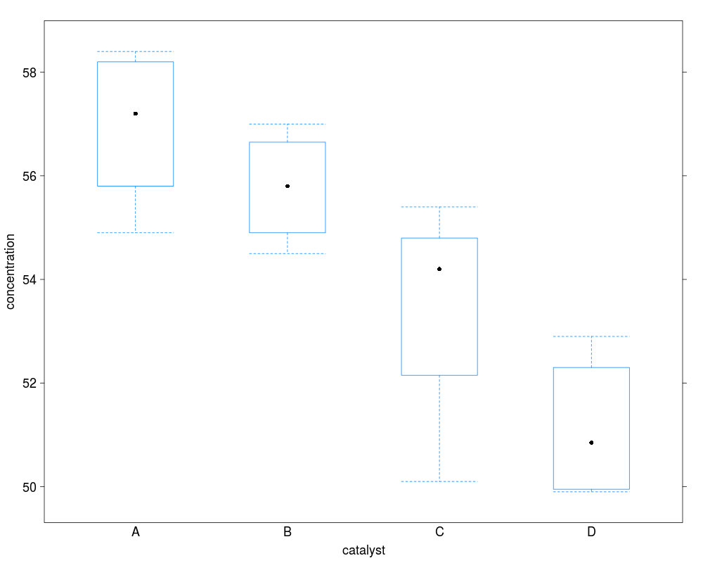
> bwplot(concent ~ catalyst, data=catalystm,
+        scales=list(cex=1.5),
+        ylab=list("concentration", cex=1.5),
+        xlab=list("catalyst",cex=1.5))
> 
> 
> catalystm1.aov <- aov(concent ~ catalyst, data=catalystm)
> summary(catalystm1.aov)
            Df Sum Sq Mean Sq F value  Pr(>F)   
catalyst     3  85.68   28.56   9.916 0.00144 **
Residuals   12  34.56    2.88                   
---
Signif. codes:  0 '***' 0.001 '**' 0.01 '*' 0.05 '.' 0.1 ' ' 1
> 
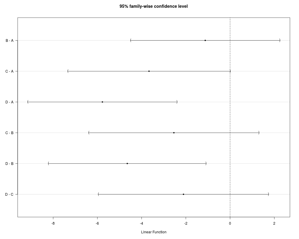
> catalystm.mca <-
+ glht(catalystm1.aov, linfct = mcp(catalyst = "Tukey"))
> confint(catalystm.mca)

	 Simultaneous Confidence Intervals

Multiple Comparisons of Means: Tukey Contrasts


Fit: aov(formula = concent ~ catalyst, data = catalystm)

Quantile = 2.9674
95% family-wise confidence level
 

Linear Hypotheses:
           Estimate lwr      upr     
B - A == 0 -1.12500 -4.50319  2.25319
C - A == 0 -3.66667 -7.34437  0.01104
D - A == 0 -5.77500 -9.15319 -2.39681
C - B == 0 -2.54167 -6.38790  1.30457
D - B == 0 -4.65000 -8.21092 -1.08908
D - C == 0 -2.10833 -5.95457  1.73790

> plot(catalystm.mca)                      ## multcomp plot
> mmcplot(catalystm.mca, focus="catalyst") ## HH plot
> 
> ## pairwise comparisons
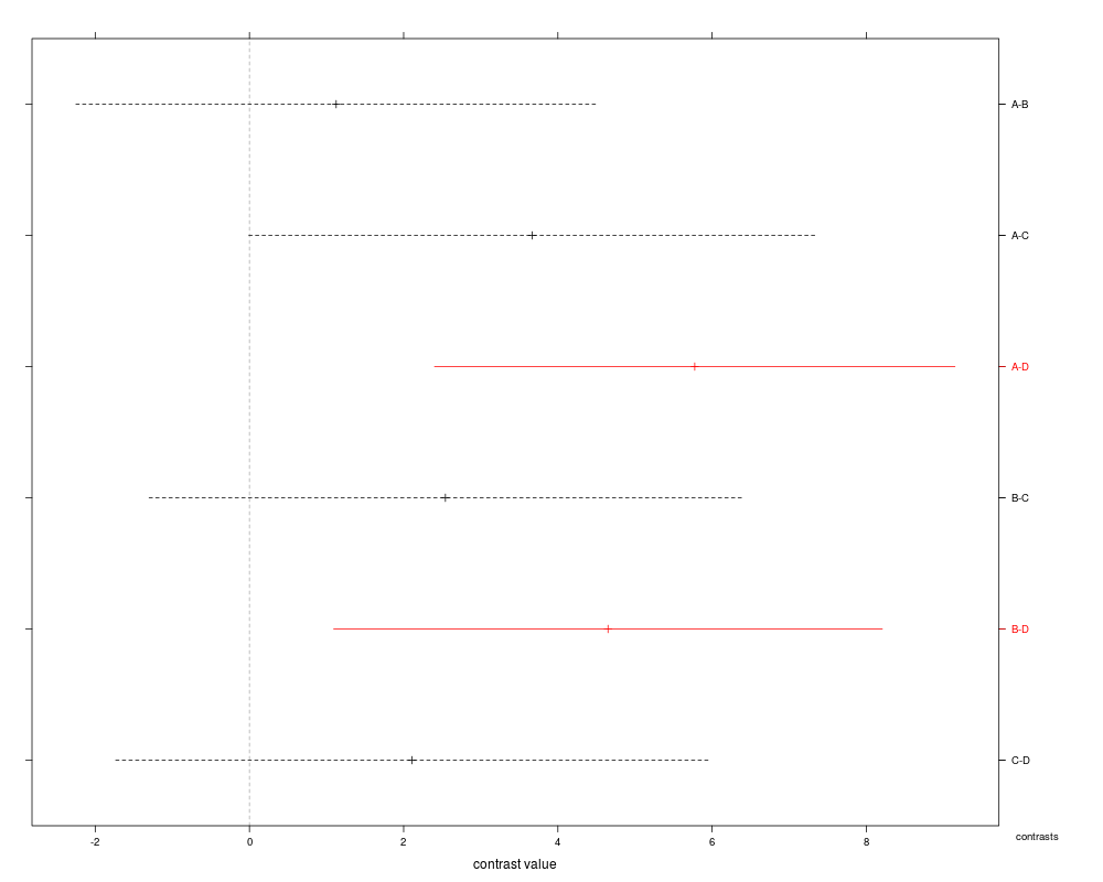
> catalystm.mmc <-
+   mmc(catalystm1.aov, focus="catalyst")
> catalystm.mmc
Tukey contrasts
Fit: aov(formula = concent ~ catalyst, data = catalystm) 
Estimated Quantile = 2.967245 
95% family-wise confidence level
$mca
    estimate   stderr      lower    upper   height
A-B 1.125000 1.138447 -2.2530523 4.503052 56.33750
A-C 3.666667 1.239385 -0.0108909 7.344224 55.06667
B-C 2.541667 1.296179 -1.3044151 6.387748 54.50417
A-D 5.775000 1.138447  2.3969477 9.153052 54.01250
B-D 4.650000 1.200029  1.0892202 8.210780 53.45000
C-D 2.108333 1.296179 -1.7377484 5.954415 52.17917
$none
  estimate    stderr    lower    upper   height
A 56.90000 0.7589649 54.64797 59.15203 56.90000
B 55.77500 0.8485486 53.25715 58.29285 55.77500
C 53.23333 0.9798195 50.32597 56.14070 53.23333
D 51.12500 0.8485486 48.60715 53.64285 51.12500
> 
> ## Not run: 
> ##D ## these three statements are identical for a one-way aov
> ##D   mmc(catalystm1.aov)  ## simplest
> ##D   mmc(catalystm1.aov, focus="catalyst") ## generalizes to higher-order designs
> ##D   mmc(catalystm1.aov, linfct = mcp(catalyst = "Tukey")) ## glht arguments
> ## End(Not run)
> 
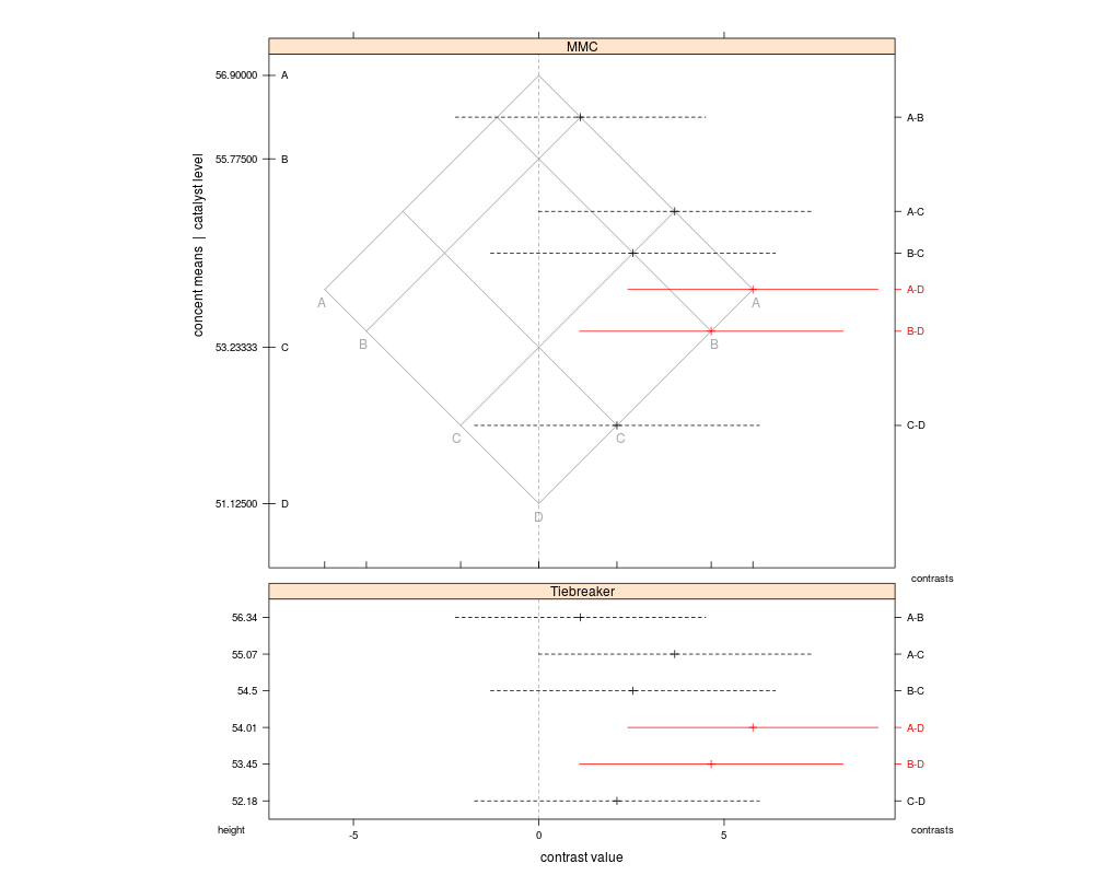
> mmcplot(catalystm.mmc, style="both")
> 
> 
> ## User-Specified Contrasts
> ## Row names must include all levels of the factor.
> ## Column names are the names the user assigns to the contrasts.
> ## Each column must sum to zero.
> catalystm.lmat <- cbind("AB-D" =c( 1, 1, 0,-2),
+                         "A-B"  =c( 1,-1, 0, 0),
+                         "ABD-C"=c( 1, 1,-3, 1))
> dimnames(catalystm.lmat)[[1]] <- levels(catalystm$catalyst)
> catalystm.lmat
  AB-D A-B ABD-C
A    1   1     1
B    1  -1     1
C    0   0    -3
D   -2   0     1
> 
> catalystm.mmc <-
+ mmc(catalystm1.aov,
+        linfct = mcp(catalyst = "Tukey"),
+        focus.lmat=catalystm.lmat)
> catalystm.mmc
Tukey contrasts
Fit: aov(formula = concent ~ catalyst, data = catalystm) 
Estimated Quantile = 2.967123 
95% family-wise confidence level
$mca
    estimate   stderr       lower    upper   height
A-B 1.125000 1.138447 -2.25291324 4.502913 56.33750
A-C 3.666667 1.239385 -0.01073948 7.344073 55.06667
B-C 2.541667 1.296179 -1.30425674 6.387590 54.50417
A-D 5.775000 1.138447  2.39708676 9.152913 54.01250
B-D 4.650000 1.200029  1.08936681 8.210633 53.45000
C-D 2.108333 1.296179 -1.73759007 5.954257 52.17917
$none
  estimate    stderr    lower    upper   height
A 56.90000 0.7589649 54.64806 59.15194 56.90000
B 55.77500 0.8485486 53.25725 58.29275 55.77500
C 53.23333 0.9798195 50.32609 56.14058 53.23333
D 51.12500 0.8485486 48.60725 53.64275 51.12500
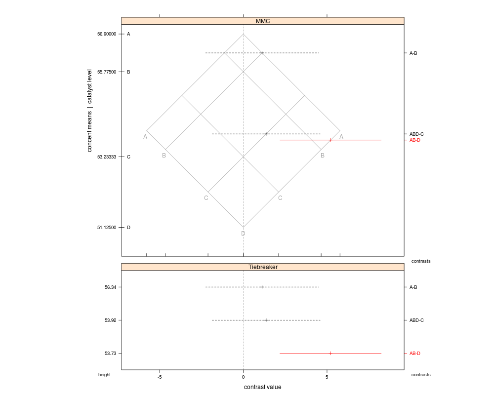
$lmat
      estimate   stderr     lower    upper   height
A-B   1.125000 1.138447 -2.252913 4.502913 56.33750
ABD-C 1.366667 1.088144 -1.861990 4.595323 53.91667
AB-D  5.212500 1.021788  2.180730 8.244270 53.73125
> 
> mmcplot(catalystm.mmc, style="both", type="lmat")
> 
> 
> ## Dunnett's test
> ## weightloss example
> data(weightloss)
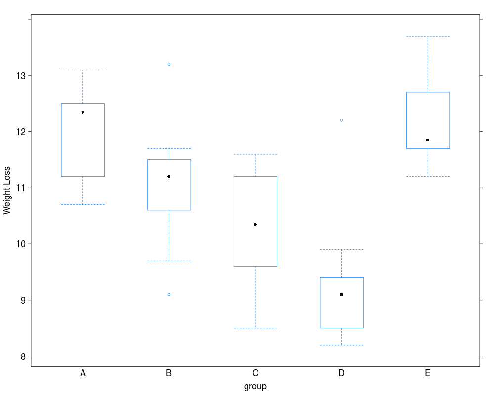
> bwplot(loss ~ group, data=weightloss,
+        scales=list(cex=1.5),
+        ylab=list("Weight Loss", cex=1.5),
+        xlab=list("group",cex=1.5))
> 
> weightloss.aov <- aov(loss ~ group, data=weightloss)
> summary(weightloss.aov)
            Df Sum Sq Mean Sq F value   Pr(>F)    
group        4  59.88  14.970   15.07 6.88e-08 ***
Residuals   45  44.70   0.993                     
---
Signif. codes:  0 '***' 0.001 '**' 0.01 '*' 0.05 '.' 0.1 ' ' 1
> 
> group.count <- table(weightloss$group)
> 
> tmp.dunnett <-
+   glht(weightloss.aov,
+        linfct=mcp(group=contrMat(group.count, base=4)),
+        alternative="greater")
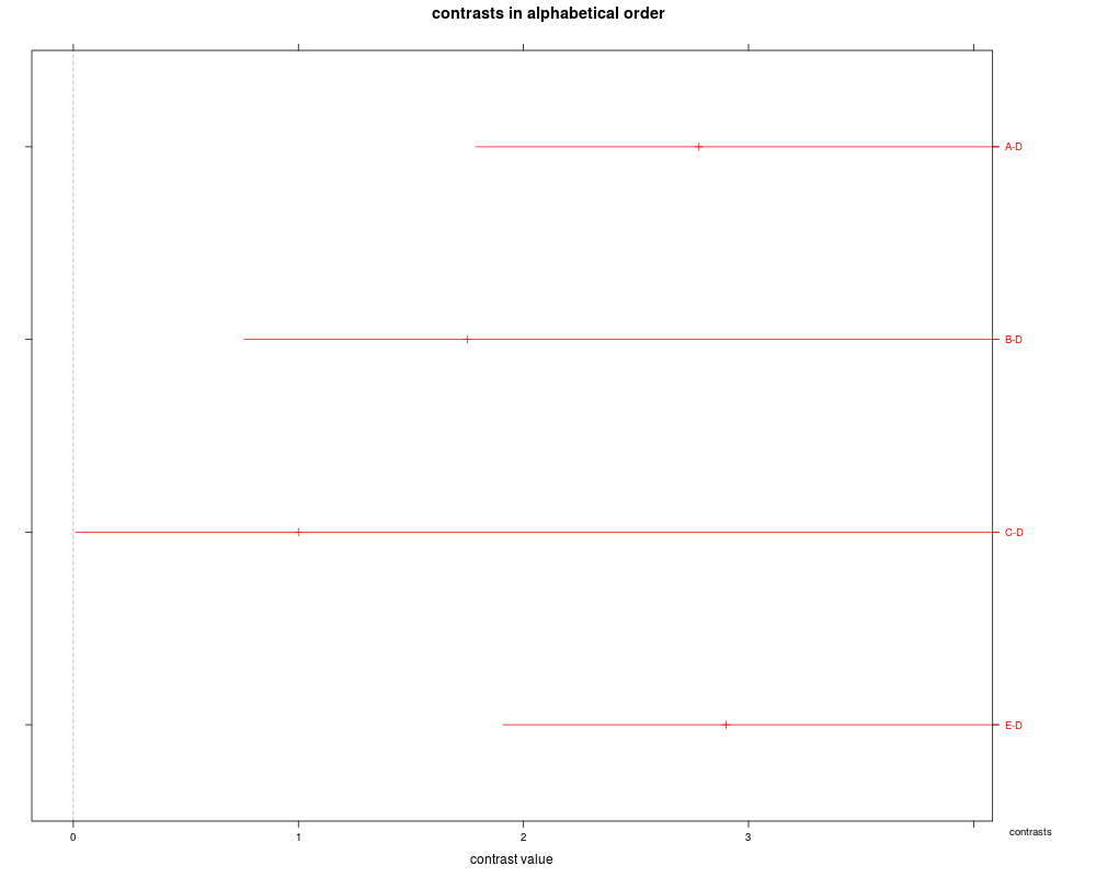
> mmcplot(tmp.dunnett, main="contrasts in alphabetical order", focus="group")
> 
> tmp.dunnett.mmc <-
+   mmc(weightloss.aov,
+       linfct=mcp(group=contrMat(group.count, base=4)),
+       alternative="greater")
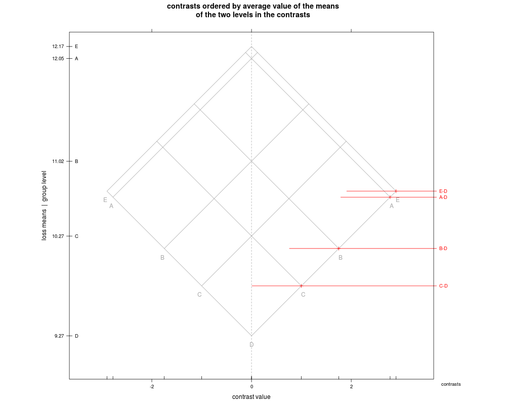
> mmcplot(tmp.dunnett.mmc,
+         main="contrasts ordered by average value of the means\nof the two levels in the contrasts")
> 
> tmp.dunnett.mmc
Dunnett contrasts
Fit: aov(formula = loss ~ group, data = weightloss) 
Estimated Quantile = -2.221557 
95% family-wise confidence level
$mca
    estimate stderr       lower upper height
E-D     2.90   -Inf 1.909762566   Inf 10.720
A-D     2.78   -Inf 1.789762566   Inf 10.660
B-D     1.75   -Inf 0.759762566   Inf 10.145
C-D     1.00   -Inf 0.009762566   Inf  9.770
$none
  estimate stderr     lower upper height
E    12.17   -Inf 11.469796   Inf  12.17
A    12.05   -Inf 11.349796   Inf  12.05
B    11.02   -Inf 10.319796   Inf  11.02
C    10.27   -Inf  9.569796   Inf  10.27
D     9.27   -Inf  8.569796   Inf   9.27
> 
> 
> ## Not run: 
> ##D ## two-way ANOVA
> ##D ## display example
> ##D 
> ##D data(display)
> ##D 
> ##D interaction2wt(time ~ emergenc * panel.ordered, data=display)
> ##D 
> ##D displayf.aov <- aov(time ~ emergenc * panel, data=display)
> ##D anova(displayf.aov)
> ##D 
> ##D ## multiple comparisons
> ##D ## MMC plot
> ##D displayf.mmc <- mmc(displayf.aov, focus="panel")
> ##D displayf.mmc
> ##D 
> ##D ## same thing using glht argument list
> ##D displayf.mmc <-
> ##D   mmc(displayf.aov,
> ##D       linfct=mcp(panel="Tukey", `interaction_average`=TRUE, `covariate_average`=TRUE))
> ##D 
> ##D mmcplot(displayf.mmc)
> ##D 
> ##D 
> ##D panel.lmat <- cbind("3-12"=c(-1,-1,2),
> ##D                     "1-2"=c( 1,-1,0))
> ##D dimnames(panel.lmat)[[1]] <- levels(display$panel)
> ##D panel.lmat
> ##D 
> ##D displayf.mmc <-
> ##D   mmc(displayf.aov, focus="panel", focus.lmat=panel.lmat)
> ##D 
> ##D ## same thing using glht argument list
> ##D displayf.mmc <-
> ##D   mmc(displayf.aov,
> ##D       linfct=mcp(panel="Tukey", `interaction_average`=TRUE, `covariate_average`=TRUE),
> ##D       focus.lmat=panel.lmat)
> ##D 
> ##D mmcplot(displayf.mmc, type="lmat")
> ## End(Not run)
> 
> ## Not run: 
> ##D ## split plot design with tiebreaker plot
> ##D ##
> ##D ## This example is based on the query by Tomas Goicoa to R-news
> ##D ## http://article.gmane.org/gmane.comp.lang.r.general/76275/match=goicoa
> ##D ## It is a split plot similar to the one in HH Section 14.2 based on
> ##D ## Yates 1937 example.  I am using the Goicoa example here because its
> ##D ## MMC plot requires a tiebreaker plot.
> ##D 
> ##D 
> ##D data(maiz)
> ##D 
> ##D interaction2wt(yield ~ hibrido+nitrogeno+bloque, data=maiz,
> ##D                par.strip.text=list(cex=.7))
> ##D interaction2wt(yield ~ hibrido+nitrogeno, data=maiz)
> ##D 
> ##D maiz.aov <- aov(yield ~ nitrogeno*hibrido + Error(bloque/nitrogeno), data=maiz)
> ##D 
> ##D summary(maiz.aov)
> ##D summary(maiz.aov,
> ##D         split=list(hibrido=list(P3732=1, Mol17=2, A632=3, LH74=4)))
> ##D 
> ##D try(glht(maiz.aov, linfct=mcp(hibrido="Tukey")))  ## can't use 'aovlist' objects in glht
> ##D 
> ##D ## R glht() requires aov, not aovlist
> ##D maiz2.aov <- aov(terms(yield ~ bloque*nitrogeno + hibrido/nitrogeno,
> ##D                        keep.order=TRUE),
> ##D                  data=maiz)
> ##D summary(maiz2.aov)
> ##D 
> ##D ## There are many ties in the group means.
> ##D ## These are easily seen in the MMC plot, where the two clusters
> ##D ## c("P3747", "P3732", "LH74") and c("Mol17", "A632")
> ##D ## are evident from the top three contrasts including zero and the
> ##D ## bottom contrast including zero.  The significant contrasts are the
> ##D ## ones comparing hybrids in the top group of three to ones in the
> ##D ## bottom group of two.
> ##D 
> ##D ## We have two graphical responses to the ties.
> ##D ## 1. We constructed the tiebreaker plot.
> ##D ## 2. We construct a set of orthogonal contrasts to illustrate
> ##D ##    the clusters.
> ##D 
> ##D ## pairwise contrasts with tiebreakers.
> ##D maiz2.mmc <- mmc(maiz2.aov,
> ##D                  linfct=mcp(hibrido="Tukey", interaction_average=TRUE))
> ##D mmcplot(maiz2.mmc, style="both")  ## MMC and Tiebreaker
> ##D 
> ##D 
> ##D ## orthogonal contrasts
> ##D ## user-specified contrasts
> ##D hibrido.lmat <- cbind("PPL-MA" =c(2, 2,-3,-3, 2),
> ##D                       "PP-L"   =c(1, 1, 0, 0,-2),
> ##D                       "P47-P32"=c(1,-1, 0, 0, 0),
> ##D                       "M-A"    =c(0, 0, 1,-1, 0))
> ##D dimnames(hibrido.lmat)[[1]] <- levels(maiz$hibrido)
> ##D hibrido.lmat
> ##D 
> ##D maiz2.mmc <-
> ##D   mmc(maiz2.aov, focus="hibrido", focus.lmat=hibrido.lmat)
> ##D maiz2.mmc
> ##D 
> ##D ## same thing using glht argument list
> ##D maiz2.mmc <-
> ##D   mmc(maiz2.aov, linfct=mcp(hibrido="Tukey",
> ##D       `interaction_average`=TRUE), focus.lmat=hibrido.lmat)
> ##D 
> ##D   mmcplot(maiz2.mmc, style="both", type="lmat")
> ## End(Not run)
> 
> 
> 
> 
> 
> dev.off()
null device 
          1 
>