Supported by Dr. Osamu Ogasawara and  . . |
|
Last data update: 2014.03.03 |
plot a normal or a t-curve with both x and z axes.DescriptionPlot a normal curve or a t-curve with both x (with When the optional argument
Usage
normal.and.t.dist(mu.H0          = 0,
                  mu.H1          = NA,
                  obs.mean       = 0,
                  std.dev        = 1,
                  n              = NA,
                  deg.freedom    = NA,
                  alpha.left     = alpha.right,
                  alpha.right    = .05,
                  Use.mu.H1      = FALSE,
                  Use.obs.mean   = FALSE,
                  Use.alpha.left = FALSE,
                  Use.alpha.right= TRUE,
                  hypoth.or.conf = 'Hypoth',
                  xmin           = NA,
                  xmax           = NA,
                  gxbar.min      = NA,
                  gxbar.max      = NA,
                  cex.crit       = 1.2,
                  polygon.density= -1,
                  polygon.lwd    = 4,
                  col.mean       = 'limegreen',
                  col.mean.label = 'limegreen',
                  col.alpha      = 'blue',
                  col.alpha.label= 'blue',
                  col.beta       = 'red',
                  col.beta.label = 'red',
                  col.conf       = 'palegreen',
                  col.conf.arrow = 'darkgreen',
                  col.conf.label = 'darkgreen'
                  )

norm.setup(xlim=c(-2.5,2.5),
           ylim = c(0, 0.4)/se,
           mean=0,
           main=main.calc,
           se=sd/sqrt(n), sd=1, n=1,
           df.t=NULL,
           Use.obs.mean=TRUE,
            ...)

norm.curve(mean=0, se=sd/sqrt(n),
          critical.values=mean + se*c(-1, 1)*z.975,
          z=if(se==0) 0 else
               do.call("seq", as.list(c((par()$usr[1:2]-mean)/se, length=109))),
          shade, col="blue",
          axis.name=ifelse(is.null(df.t) || df.t==Inf, "z", "t"),
          second.axis.label.line=3,
          sd=1, n=1,
          df.t=NULL,
          axis.name.expr=axis.name,
          Use.obs.mean=TRUE,
          col.label=col,
          hypoth.or.conf="Hypoth",
          col.conf.arrow=par("col"),
          col.conf.label=par("col"),
          col.crit=ifelse(hypoth.or.conf=="Hypoth", 'blue', col.conf.arrow),
          cex.crit=1.2,
          polygon.density=-1,
          polygon.lwd=4,
          col.border=ifelse(is.na(polygon.density), FALSE, col),
          ...)

norm.observed(xbar, t.xbar, t.xbar.H1=NULL,
              col="green",
              p.val=NULL, p.val.x=par()$usr[2]+ left.margin,
              t.or.z=ifelse(is.null(deg.free) || deg.free==Inf, "z", "t"),
              t.or.z.position=par()$usr[1]-left.margin,
              cex.small=par()$cex*.7, col.label=col,
              xbar.negt=NULL, cex.large=par()$cex,
              left.margin=.15*diff(par()$usr[1:2]),
              sided="", deg.free=NULL)

norm.outline(dfunction, left, right, mu.H0, se, deg.free=NULL,
             col.mean="green")
Arguments
ValueAn invisible list containing the
calculated values of probabilities and critical values in the data
scale, the null hypothesis z- or t-scale, and the alternative
hypothesis z- or t-scale, as specified. The components are:
Author(s)Richard M. Heiberger <rmh@temple.edu> Examples
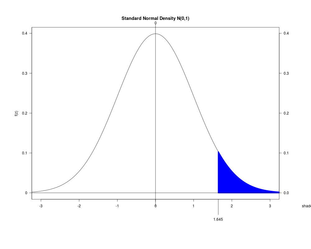
normal.and.t.dist()
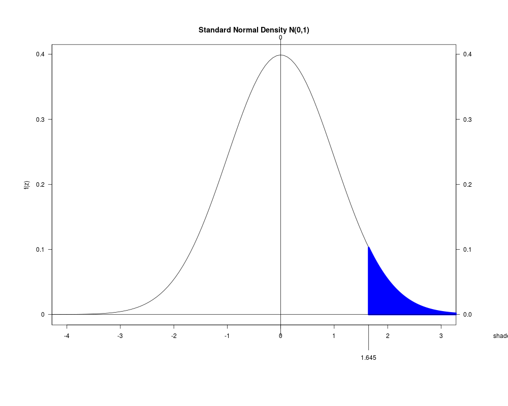
normal.and.t.dist(xmin=-4)
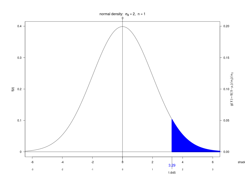
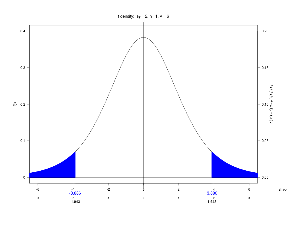
normal.and.t.dist(std.dev=2)
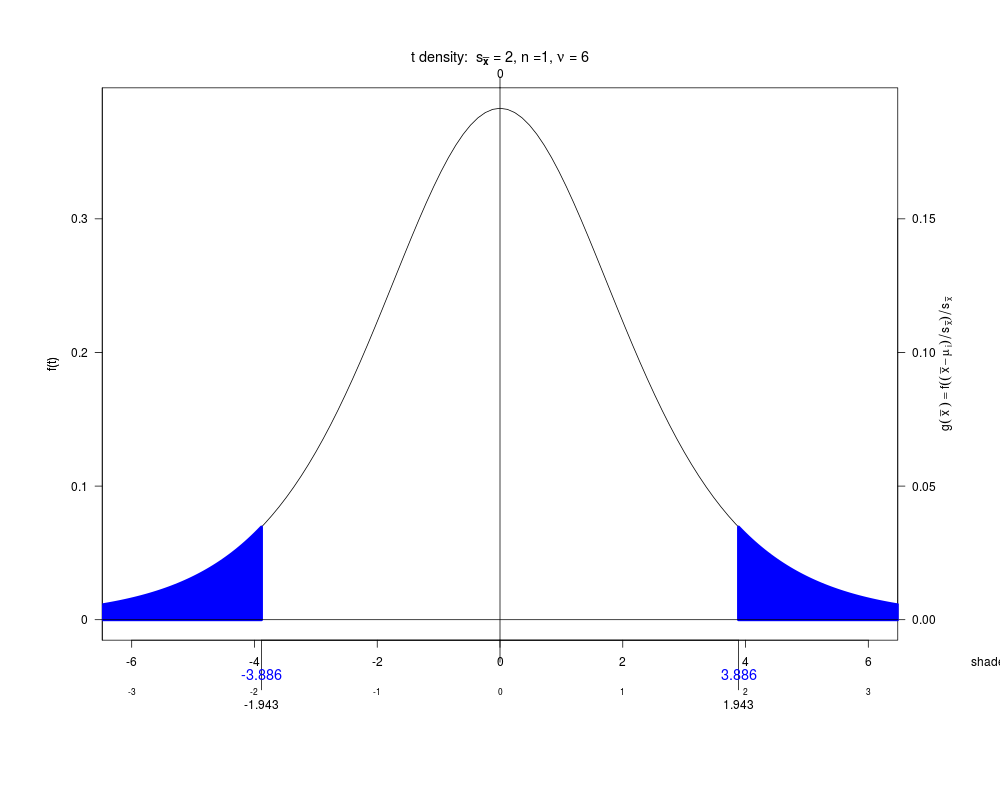
normal.and.t.dist(std.dev=2, Use.alpha.left=TRUE, deg.free=6)
normal.and.t.dist(std.dev=2, Use.alpha.left=TRUE, deg.free=6, gxbar.max=.20)
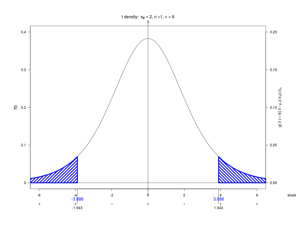
normal.and.t.dist(std.dev=2, Use.alpha.left=TRUE, deg.free=6,
gxbar.max=.20, polygon.density=10)
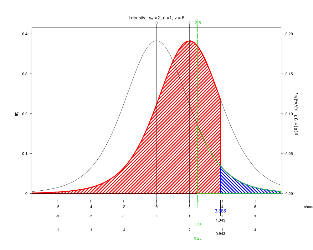
normal.and.t.dist(std.dev=2, Use.alpha.left=FALSE, deg.free=6,
gxbar.max=.20, polygon.density=10,
mu.H1=2, Use.mu.H1=TRUE,
obs.mean=2.5, Use.obs.mean=TRUE, xmin=-7)
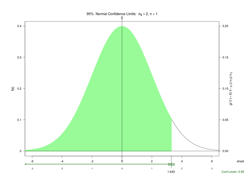
normal.and.t.dist(std.dev=2, hypoth.or.conf="Conf")
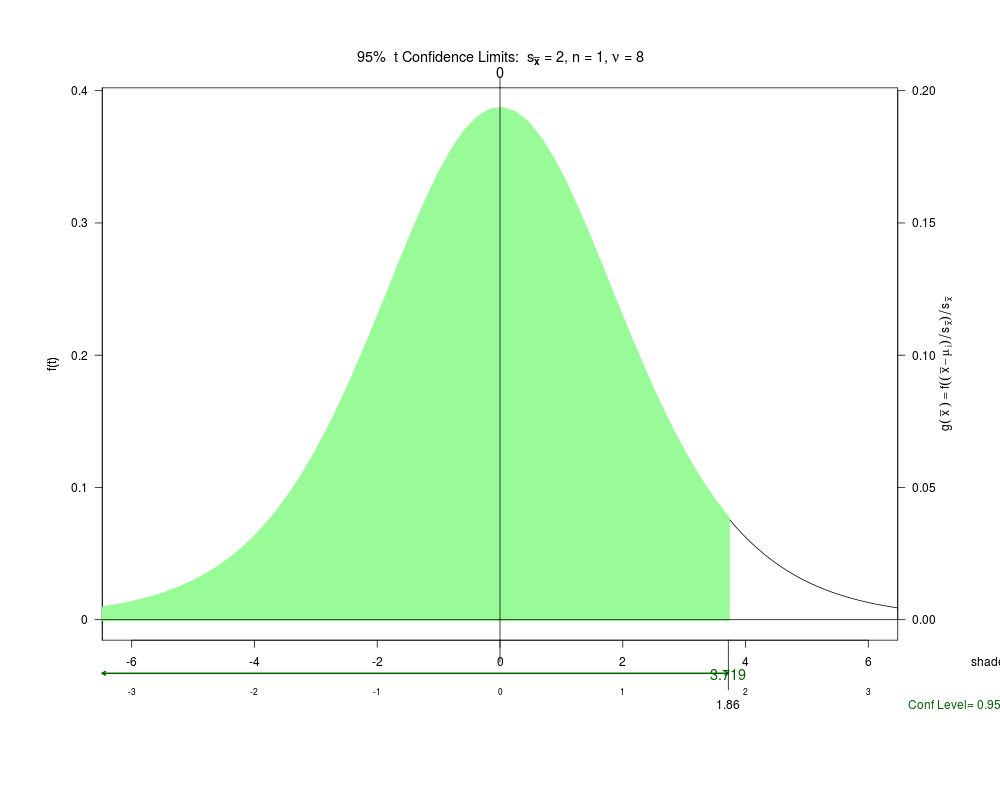
normal.and.t.dist(std.dev=2, hypoth.or.conf="Conf", deg.free=8)
old.par <- par(oma=c(4,0,2,5), mar=c(7,7,4,2)+.1)
norm.setup()
norm.curve()
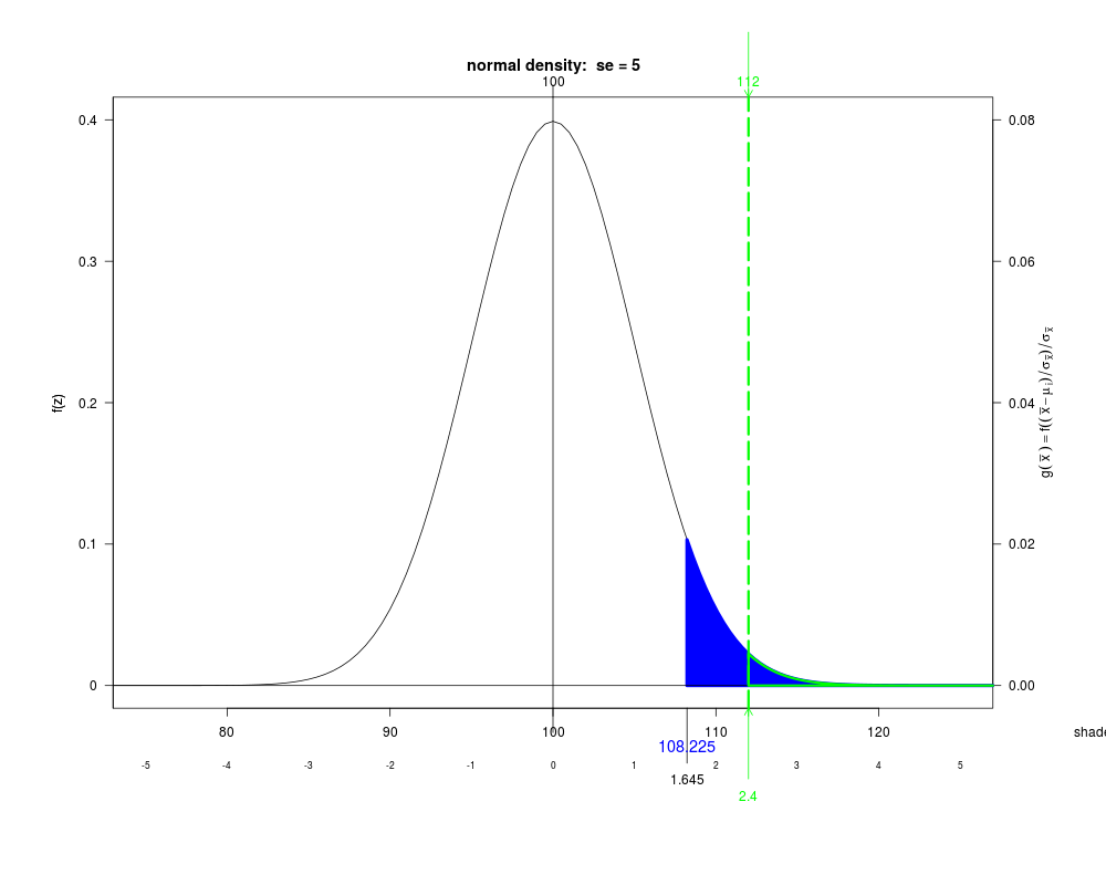
norm.setup(xlim=c(75,125), mean=100, se=5)
norm.curve(100, 5, 100+5*(1.645))
norm.observed(112, (112-100)/5)
norm.outline("dnorm", 112, par()$usr[2], 100, 5)
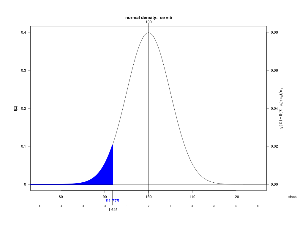
norm.setup(xlim=c(75,125), mean=100, se=5)
norm.curve(100, 5, 100+5*(-1.645), shade="left")
norm.setup(xlim=c(75,125), mean=100, se=5)
norm.curve(mean=100, se=5, col='red')
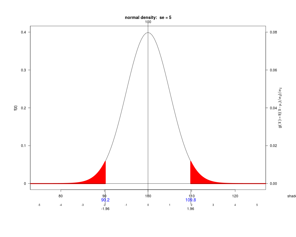
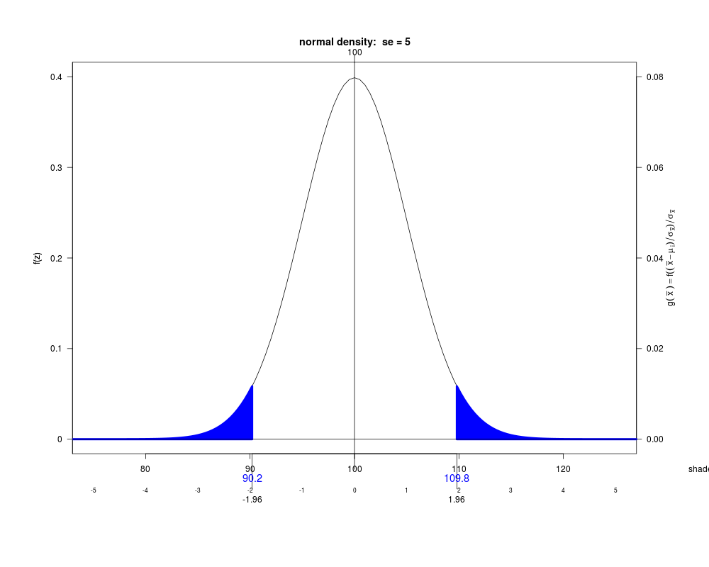
norm.setup(xlim=c(75,125), mean=100, se=5)
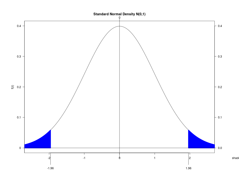
norm.curve(100, 5, 100+5*c(-1.96, 1.96))
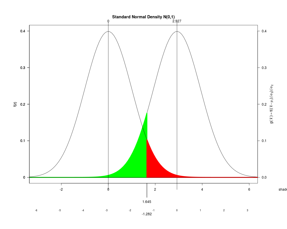
norm.setup(xlim=c(-3, 6))
norm.curve(critical.values=1.645, mean=1.645+1.281552, col='green',
shade="left", axis.name="z1")
norm.curve(critical.values=1.645, col='red')
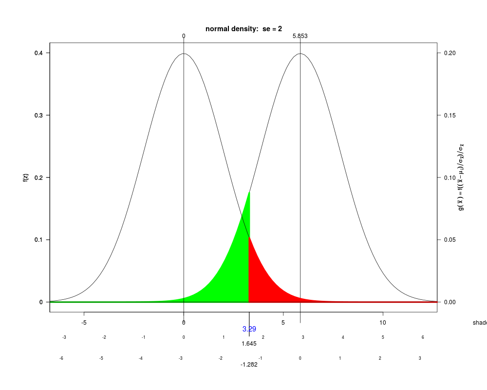
norm.setup(xlim=c(-6, 12), se=2)
norm.curve(critical.values=2*1.645, se=2, mean=2*(1.645+1.281552),
col='green', shade="left", axis.name="z1")
norm.curve(critical.values=2*1.645, se=2, mean=0,
col='red', shade="right")
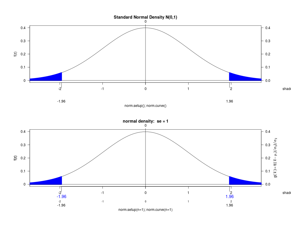
par(mfrow=c(2,1))
norm.setup()
norm.curve()
mtext("norm.setup(); norm.curve()", side=1, line=5)
norm.setup(n=1)
norm.curve(n=1)
mtext("norm.setup(n=1); norm.curve(n=1)", side=1, line=5)
par(mfrow=c(1,1))
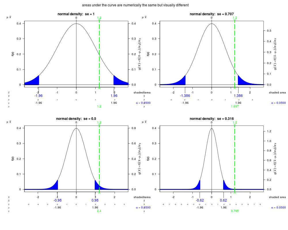
par(mfrow=c(2,2))
## naively scaled,
## areas under the curve are numerically the same but visually different
norm.setup(n=1)
norm.curve(n=1)
norm.observed(1.2, 1.2/(1/sqrt(1)))
norm.setup(n=2)
norm.curve(n=2)
norm.observed(1.2, 1.2/(1/sqrt(2)))
norm.setup(n=4)
norm.curve(n=4)
norm.observed(1.2, 1.2/(1/sqrt(4)))
norm.setup(n=10)
norm.curve(n=10)
norm.observed(1.2, 1.2/(1/sqrt(10)))
mtext("areas under the curve are numerically the same but visually different",
side=3, outer=TRUE)
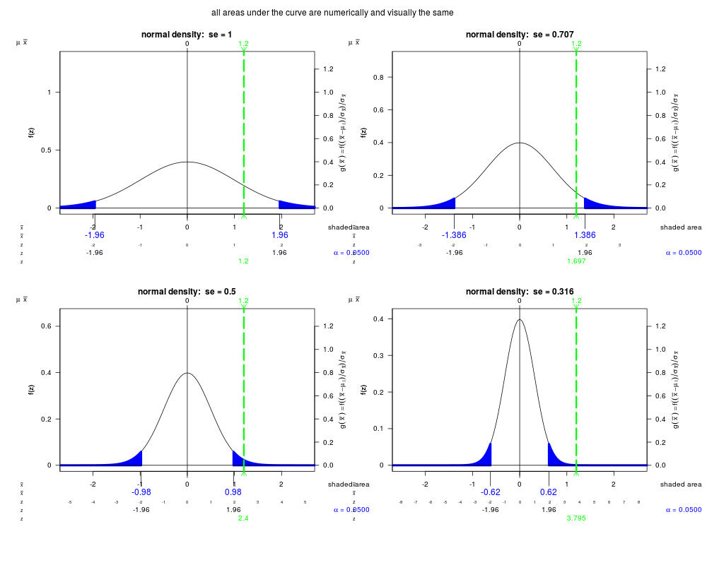
## scaled so all areas under the curve are numerically and visually the same
norm.setup(n=1, ylim=c(0,1.3))
norm.curve(n=1)
norm.observed(1.2, 1.2/(1/sqrt(1)))
norm.setup(n=2, ylim=c(0,1.3))
norm.curve(n=2)
norm.observed(1.2, 1.2/(1/sqrt(2)))
norm.setup(n=4, ylim=c(0,1.3))
norm.curve(n=4)
norm.observed(1.2, 1.2/(1/sqrt(4)))
norm.setup(n=10, ylim=c(0,1.3))
norm.curve(n=10)
norm.observed(1.2, 1.2/(1/sqrt(10)))
mtext("all areas under the curve are numerically and visually the same",
side=3, outer=TRUE)
par(mfrow=c(1,1))
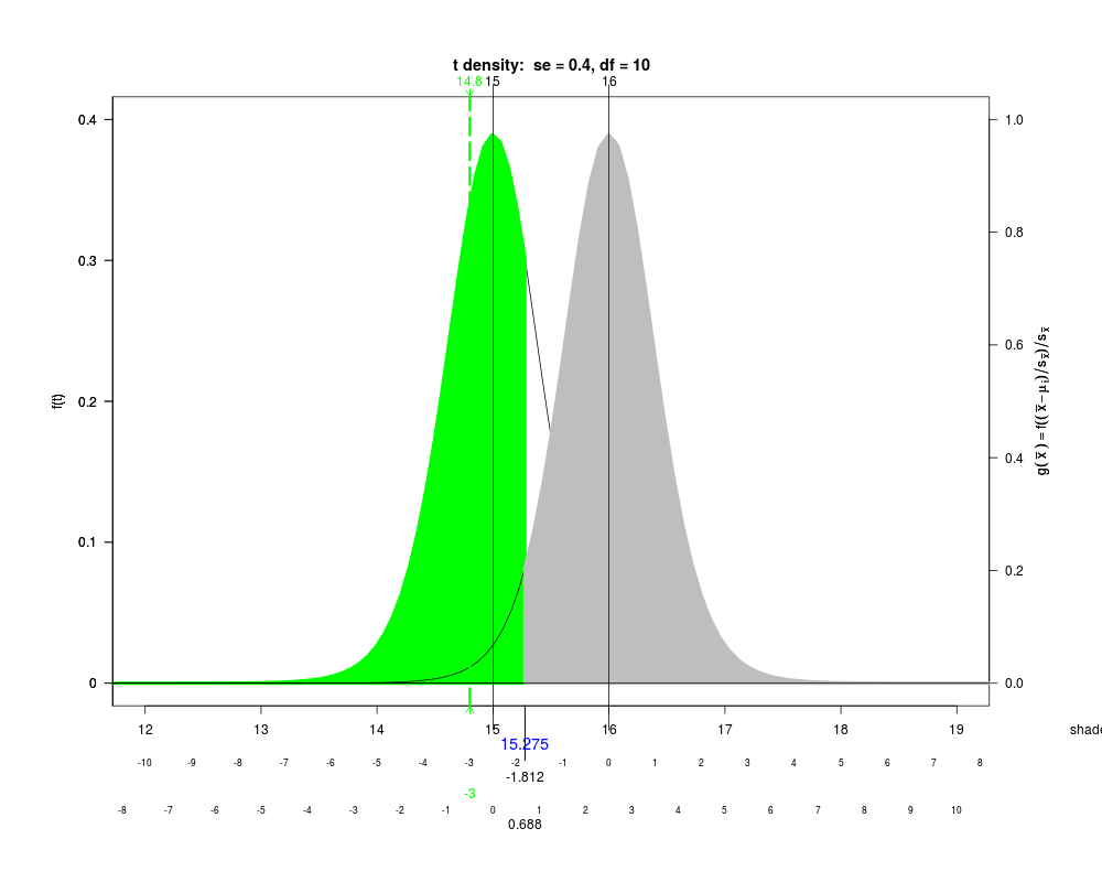
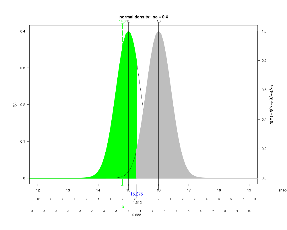
## t distribution
mu.H0 <- 16
se.val <- .4
df.val <- 10
crit.val <- mu.H0 - qt(.95, df.val) * se.val
mu.alt <- 15
obs.mean <- 14.8
alt.t <- (mu.alt - crit.val) / se.val
norm.setup(xlim=c(12, 19), se=se.val, df.t=df.val)
norm.curve(critical.values=crit.val, se=se.val, df.t=df.val, mean=mu.alt,
col='green', shade="left", axis.name="t1")
norm.curve(critical.values=crit.val, se=se.val, df.t=df.val, mean=mu.H0,
col='gray', shade="right")
norm.observed(obs.mean, (obs.mean-mu.H0)/se.val)
## normal
norm.setup(xlim=c(12, 19), se=se.val)
norm.curve(critical.values=crit.val, se=se.val, mean=mu.alt,
col='green', shade="left", axis.name="z1")
norm.curve(critical.values=crit.val, se=se.val, mean=mu.H0,
col='gray', shade="right")
norm.observed(obs.mean, (obs.mean-mu.H0)/se.val)
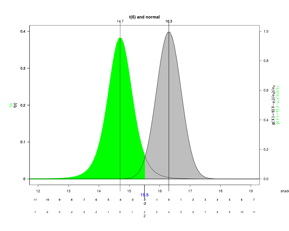
## normal and t
norm.setup(xlim=c(12, 19), se=se.val, main="t(6) and normal")
norm.curve(critical.values=15.5, se=se.val, mean=16.3,
col='gray', shade="right")
norm.curve(critical.values=15.5, se.val, df.t=6, mean=14.7,
col='green', shade="left", axis.name="t1", second.axis.label.line=4)
norm.curve(critical.values=15.5, se=se.val, mean=16.3,
col='gray', shade="none")
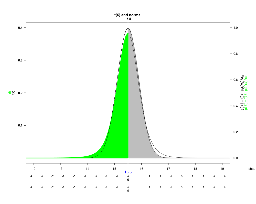
norm.setup(xlim=c(12, 19), se=se.val, main="t(6) and normal")
norm.curve(critical.values=15.5, se=se.val, mean=15.5,
col='gray', shade="right")
norm.curve(critical.values=15.5, se=se.val, df.t=6, mean=15.5,
col='green', shade="left", axis.name="t1", second.axis.label.line=4)
norm.curve(critical.values=15.5, se=se.val, mean=15.5,
col='gray', shade="none")
par(old.par)
Results
R version 3.3.1 (2016-06-21) -- "Bug in Your Hair"
Copyright (C) 2016 The R Foundation for Statistical Computing
Platform: x86_64-pc-linux-gnu (64-bit)

R is free software and comes with ABSOLUTELY NO WARRANTY.
You are welcome to redistribute it under certain conditions.
Type 'license()' or 'licence()' for distribution details.

R is a collaborative project with many contributors.
Type 'contributors()' for more information and
'citation()' on how to cite R or R packages in publications.

Type 'demo()' for some demos, 'help()' for on-line help, or
'help.start()' for an HTML browser interface to help.
Type 'q()' to quit R.

> library(HH)
Loading required package: lattice
Loading required package: grid
Loading required package: latticeExtra
Loading required package: RColorBrewer
Loading required package: multcomp
Loading required package: mvtnorm
Loading required package: survival
Loading required package: TH.data
Loading required package: MASS

Attaching package: 'TH.data'

The following object is masked from 'package:MASS':

    geyser

Loading required package: gridExtra
> png(filename="/home/ddbj/snapshot/RGM3/R_CC/result/HH/norm.curve.Rd_%03d_medium.png", width=480, height=480)
> ### Name: norm.curve
> ### Title: plot a normal or a t-curve with both x and z axes.
> ### Aliases: norm.setup norm.curve norm.observed norm.outline
> ###   normal.and.t.dist
> ### Keywords: aplot hplot distribution
>
> ### ** Examples
>
> normal.and.t.dist()
> normal.and.t.dist(xmin=-4)
> normal.and.t.dist(std.dev=2)
> normal.and.t.dist(std.dev=2, Use.alpha.left=TRUE, deg.free=6)
> normal.and.t.dist(std.dev=2, Use.alpha.left=TRUE, deg.free=6, gxbar.max=.20)
> normal.and.t.dist(std.dev=2, Use.alpha.left=TRUE, deg.free=6,
+                   gxbar.max=.20, polygon.density=10)
> normal.and.t.dist(std.dev=2, Use.alpha.left=FALSE, deg.free=6,
+                   gxbar.max=.20, polygon.density=10,
+                   mu.H1=2, Use.mu.H1=TRUE,
+                   obs.mean=2.5, Use.obs.mean=TRUE, xmin=-7)
> normal.and.t.dist(std.dev=2, hypoth.or.conf="Conf")
> normal.and.t.dist(std.dev=2, hypoth.or.conf="Conf", deg.free=8)
>
> old.par <- par(oma=c(4,0,2,5), mar=c(7,7,4,2)+.1)
>
> norm.setup()
> norm.curve()
>
> norm.setup(xlim=c(75,125), mean=100, se=5)
> norm.curve(100, 5, 100+5*(1.645))
> norm.observed(112, (112-100)/5)
> norm.outline("dnorm", 112, par()$usr[2], 100, 5)
>
> norm.setup(xlim=c(75,125), mean=100, se=5)
> norm.curve(100, 5, 100+5*(-1.645), shade="left")
>
> norm.setup(xlim=c(75,125), mean=100, se=5)
> norm.curve(mean=100, se=5, col='red')
>
> norm.setup(xlim=c(75,125), mean=100, se=5)
> norm.curve(100, 5, 100+5*c(-1.96, 1.96))
>
> norm.setup(xlim=c(-3, 6))
> norm.curve(critical.values=1.645, mean=1.645+1.281552, col='green',
+            shade="left", axis.name="z1")
> norm.curve(critical.values=1.645, col='red')
>
> norm.setup(xlim=c(-6, 12), se=2)
> norm.curve(critical.values=2*1.645, se=2, mean=2*(1.645+1.281552),
+            col='green', shade="left", axis.name="z1")
> norm.curve(critical.values=2*1.645, se=2, mean=0,
+            col='red', shade="right")
>
>
> par(mfrow=c(2,1))
> norm.setup()
> norm.curve()
> mtext("norm.setup(); norm.curve()", side=1,  line=5)
> norm.setup(n=1)
> norm.curve(n=1)
> mtext("norm.setup(n=1); norm.curve(n=1)", side=1,  line=5)
> par(mfrow=c(1,1))
>
>
> par(mfrow=c(2,2))
>
> ## naively scaled,
> ## areas under the curve are numerically the same but visually different
> norm.setup(n=1)
> norm.curve(n=1)
> norm.observed(1.2, 1.2/(1/sqrt(1)))
> norm.setup(n=2)
> norm.curve(n=2)
> norm.observed(1.2, 1.2/(1/sqrt(2)))
> norm.setup(n=4)
> norm.curve(n=4)
> norm.observed(1.2, 1.2/(1/sqrt(4)))
> norm.setup(n=10)
> norm.curve(n=10)
> norm.observed(1.2, 1.2/(1/sqrt(10)))
> mtext("areas under the curve are numerically the same but visually different",
+       side=3, outer=TRUE)
>
> ## scaled so all areas under the curve are numerically and visually the same
> norm.setup(n=1, ylim=c(0,1.3))
> norm.curve(n=1)
> norm.observed(1.2, 1.2/(1/sqrt(1)))
> norm.setup(n=2, ylim=c(0,1.3))
> norm.curve(n=2)
> norm.observed(1.2, 1.2/(1/sqrt(2)))
> norm.setup(n=4, ylim=c(0,1.3))
> norm.curve(n=4)
> norm.observed(1.2, 1.2/(1/sqrt(4)))
> norm.setup(n=10, ylim=c(0,1.3))
> norm.curve(n=10)
> norm.observed(1.2, 1.2/(1/sqrt(10)))
> mtext("all areas under the curve are numerically and visually the same",
+       side=3, outer=TRUE)
>
> par(mfrow=c(1,1))
>
>
> ## t distribution
> mu.H0 <- 16
> se.val <- .4
> df.val <- 10
> crit.val <- mu.H0 - qt(.95, df.val) * se.val
> mu.alt <- 15
> obs.mean <- 14.8
>
> alt.t <- (mu.alt - crit.val) / se.val
> norm.setup(xlim=c(12, 19), se=se.val, df.t=df.val)
> norm.curve(critical.values=crit.val, se=se.val, df.t=df.val, mean=mu.alt,
+            col='green', shade="left", axis.name="t1")
> norm.curve(critical.values=crit.val, se=se.val, df.t=df.val, mean=mu.H0,
+            col='gray', shade="right")
> norm.observed(obs.mean, (obs.mean-mu.H0)/se.val)
>
> ## normal
> norm.setup(xlim=c(12, 19), se=se.val)
> norm.curve(critical.values=crit.val, se=se.val, mean=mu.alt,
+            col='green', shade="left", axis.name="z1")
> norm.curve(critical.values=crit.val, se=se.val, mean=mu.H0,
+            col='gray', shade="right")
> norm.observed(obs.mean, (obs.mean-mu.H0)/se.val)
>
>
>
> ## normal and t
> norm.setup(xlim=c(12, 19), se=se.val, main="t(6) and normal")
> norm.curve(critical.values=15.5, se=se.val, mean=16.3,
+            col='gray', shade="right")
> norm.curve(critical.values=15.5, se.val, df.t=6, mean=14.7,
+            col='green', shade="left", axis.name="t1", second.axis.label.line=4)
> norm.curve(critical.values=15.5, se=se.val, mean=16.3,
+            col='gray', shade="none")
>
> norm.setup(xlim=c(12, 19), se=se.val, main="t(6) and normal")
> norm.curve(critical.values=15.5, se=se.val, mean=15.5,
+            col='gray', shade="right")
> norm.curve(critical.values=15.5, se=se.val, df.t=6, mean=15.5,
+            col='green', shade="left", axis.name="t1", second.axis.label.line=4)
> norm.curve(critical.values=15.5, se=se.val, mean=15.5,
+            col='gray', shade="none")
>
>
>
> par(old.par)
>
>
>
>
>
> dev.off()
null device
          1
>
|