MMC (Mean–mean Multiple Comparisons) plot.

Description

MMC (Mean–mean Multiple Comparisons) plot. The plot method documented here is no longer recommended for R; use mmcplot instead. This method is still necessary for S-Plus.

Usage

## S3 method for class 'mmc.multicomp'
plot(x,
     xlab="contrast value",
     ylab=none$ylabel,
     focus=none$focus,
     main= main.method.phrase,
     main2=main2.method.phrase,
     main.method.phrase=
       paste("multiple comparisons of means of", ylab),
     main2.method.phrase=paste("simultaneous ",
       100*(1-none$alpha),"% confidence limits, ",
       method, " method", sep="" ),
     ry.mmc=TRUE,
     key.x=par()$usr[1]+ diff(par()$usr[1:2])/20,
     key.y=par()$usr[3]+ diff(par()$usr[3:4])/3,
     method=if (is.null(mca)) lmat$method else mca$method,
     print.lmat=(!is.null(lmat)),
     print.mca=(!is.null(mca) && (!print.lmat)),
     iso.name=TRUE,
     x.offset=0,
     col.mca.signif="red",  col.mca.not.signif="black",
     lty.mca.signif=1,  lty.mca.not.signif=6,
     lwd.mca.signif=1,  lwd.mca.not.signif=1,
     col.lmat.signif="blue", col.lmat.not.signif="black",
     lty.lmat.signif=1, lty.lmat.not.signif=6,
     lwd.lmat.signif=1, lwd.lmat.not.signif=1,
     lty.iso=7, col.iso="darkgray", lwd.iso=1,
     lty.contr0=2, col.contr0="darkgray", lwd.contr0=1,
     decdigits.ybar=2,
     ...
     )

Arguments

Note

plot.mmc.multicomp chooses sensible defaults for its many arguments. They will often need manual adjustment. The examples show several types of adjustments. We have changed the centering and scaling to avoid overprinting of label information. By default the significant contrasts are shown in a more intense color than the nonsignificant contrasts. We have an option to reduce the color intensity of the isomeans grid.

When there is overprinting of labels (a consequence of level means being close together), a tiebreaker plot may be needed. See ?MMC for an example.

Author(s)

Richard M. Heiberger <rmh@temple.edu>

References

Heiberger, Richard M. and Holland, Burt (2004b). Statistical Analysis and Data Display: An Intermediate Course with Examples in S-Plus, R, and SAS. Springer Texts in Statistics. Springer. ISBN 0-387-40270-5.

Heiberger, Richard M. and Holland, Burt (2006). "Mean–mean multiple comparison displays for families of linear contrasts." Journal of Computational and Graphical Statistics, 15:937–955.

Hsu, J. and Peruggia, M. (1994). "Graphical representations of Tukey's multiple comparison method." Journal of Computational and Graphical Statistics, 3:143–161.

See Also

mmc, plotMatchMMC, mmcplot.

Examples

data(catalystm)
catalystm1.aov <- aov(concent ~ catalyst, data=catalystm)
summary(catalystm1.aov)

## See ?MMC to see why these contrasts are chosen
catalystm.lmat <- cbind("AB-D" =c( 1, 1, 0,-2),
                        "A-B"  =c( 1,-1, 0, 0),
                        "ABD-C"=c( 1, 1,-3, 1))
dimnames(catalystm.lmat)[[1]] <- levels(catalystm$catalyst)


catalystm.mmc <-
if.R(r={mmc(catalystm1.aov, linfct = mcp(catalyst = "Tukey"),
            focus.lmat=catalystm.lmat)}
    ,s={multicomp.mmc(catalystm1.aov, focus.lmat=catalystm.lmat,
                     plot=FALSE)}
)

## Not run: 
## pairwise contrasts, default settings
plot(catalystm.mmc, print.lmat=FALSE)

## End(Not run)

## Centering, scaling, emphasize significant contrasts.
## Needed in R with 7in x 7in default plot window.
## Not needed in S-Plus with 4x3 aspect ratio of plot window.
plot(catalystm.mmc, x.offset=2.1, ry.mmc=c(50,58), print.lmat=FALSE)

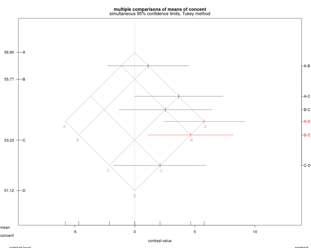
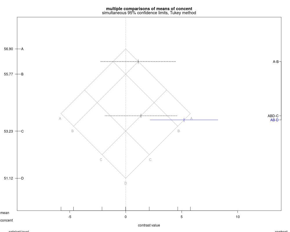
## user-specified contrasts
plot(catalystm.mmc, x.offset=2.1, ry.mmc=c(50,58))

## reduce intensity of isomeans grid, number isomeans grid lines
plot(catalystm.mmc, x.offset=2.1, ry.mmc=c(50,58),
     lty.iso=2, col.iso='darkgray', iso.name=FALSE)

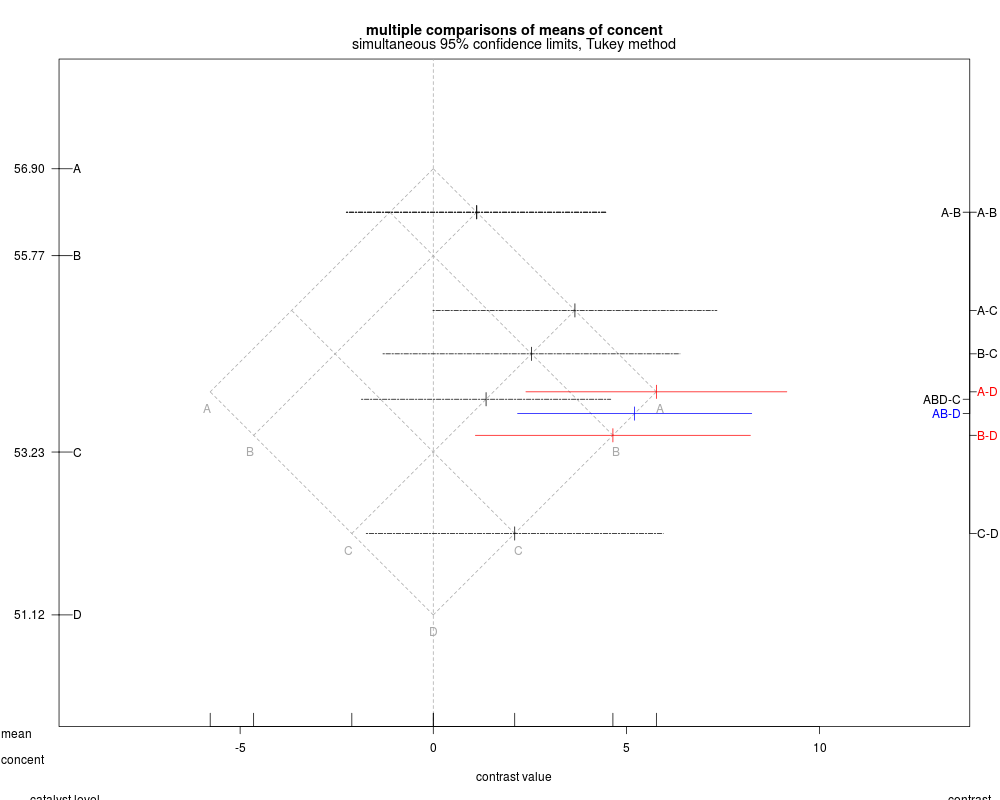
## both pairwise contrasts and user-specified contrasts
plot(catalystm.mmc, x.offset=2.1, ry.mmc=c(50,58), lty.iso=2,
     col.iso='darkgray', print.mca=TRUE)

## Not run: 
## newer mmcplot
mmcplot(catalystm.mmc)
mmcplot(catalystm.mmc, type="lmat")

## End(Not run)

Results

R version 3.3.1 (2016-06-21) -- "Bug in Your Hair"
Copyright (C) 2016 The R Foundation for Statistical Computing
Platform: x86_64-pc-linux-gnu (64-bit)

R is free software and comes with ABSOLUTELY NO WARRANTY.
You are welcome to redistribute it under certain conditions.
Type 'license()' or 'licence()' for distribution details.

R is a collaborative project with many contributors.
Type 'contributors()' for more information and
'citation()' on how to cite R or R packages in publications.

Type 'demo()' for some demos, 'help()' for on-line help, or
'help.start()' for an HTML browser interface to help.
Type 'q()' to quit R.

> library(HH)
Loading required package: lattice
Loading required package: grid
Loading required package: latticeExtra
Loading required package: RColorBrewer
Loading required package: multcomp
Loading required package: mvtnorm
Loading required package: survival
Loading required package: TH.data
Loading required package: MASS

Attaching package: 'TH.data'

The following object is masked from 'package:MASS':

    geyser

Loading required package: gridExtra
> png(filename="/home/ddbj/snapshot/RGM3/R_CC/result/HH/plot.mmc.multicomp.Rd_%03d_medium.png", width=480, height=480)
> ### Name: plot.mmc.multicomp
> ### Title: MMC (Mean-mean Multiple Comparisons) plot.
> ### Aliases: plot.mmc.multicomp
> ### Keywords: hplot
> 
> ### ** Examples
> 
> data(catalystm)
> catalystm1.aov <- aov(concent ~ catalyst, data=catalystm)
> summary(catalystm1.aov)
            Df Sum Sq Mean Sq F value  Pr(>F)   
catalyst     3  85.68   28.56   9.916 0.00144 **
Residuals   12  34.56    2.88                   
---
Signif. codes:  0 '***' 0.001 '**' 0.01 '*' 0.05 '.' 0.1 ' ' 1
> 
> ## See ?MMC to see why these contrasts are chosen
> catalystm.lmat <- cbind("AB-D" =c( 1, 1, 0,-2),
+                         "A-B"  =c( 1,-1, 0, 0),
+                         "ABD-C"=c( 1, 1,-3, 1))
> dimnames(catalystm.lmat)[[1]] <- levels(catalystm$catalyst)
> 
> 
> catalystm.mmc <-
+ if.R(r={mmc(catalystm1.aov, linfct = mcp(catalyst = "Tukey"),
+             focus.lmat=catalystm.lmat)}
+     ,s={multicomp.mmc(catalystm1.aov, focus.lmat=catalystm.lmat,
+                      plot=FALSE)}
+ )
> 
> ## Not run: 
> ##D ## pairwise contrasts, default settings
> ##D plot(catalystm.mmc, print.lmat=FALSE)
> ## End(Not run)
> 
> ## Centering, scaling, emphasize significant contrasts.
> ## Needed in R with 7in x 7in default plot window.
> ## Not needed in S-Plus with 4x3 aspect ratio of plot window.
> plot(catalystm.mmc, x.offset=2.1, ry.mmc=c(50,58), print.lmat=FALSE)
> 
> ## user-specified contrasts
> plot(catalystm.mmc, x.offset=2.1, ry.mmc=c(50,58))
> 
> ## reduce intensity of isomeans grid, number isomeans grid lines
> plot(catalystm.mmc, x.offset=2.1, ry.mmc=c(50,58),
+      lty.iso=2, col.iso='darkgray', iso.name=FALSE)
> 
> ## both pairwise contrasts and user-specified contrasts
> plot(catalystm.mmc, x.offset=2.1, ry.mmc=c(50,58), lty.iso=2,
+      col.iso='darkgray', print.mca=TRUE)
> 
> ## Not run: 
> ##D ## newer mmcplot
> ##D mmcplot(catalystm.mmc)
> ##D mmcplot(catalystm.mmc, type="lmat")
> ## End(Not run)
> 
> 
> 
> 
> 
> dev.off()
null device 
          1 
>