R Graphical Manual

Browse All

Last data update: 2014.03.03

R: plot x and y, with optional straight line fit and display of...

regr1.plot

R Documentation

plot x and y, with optional straight line fit and display of squared residuals

Description

Plot x and y, with optional fitted line and display of squared residuals. By default the least squares line is calculated and used. Any other straight line can be specified by placing its coefficients in coef.model. Any other fitted model can be calculated by specifying the model argument. Any other function of one variable can be specified in the alt.function argument. At most one of the arguments model, coef.model, alt.function can be specified.

Usage

regr1.plot(x, y,
           model=lm(y~x),
           coef.model,
           alt.function,
           main="put a useful title here",
           xlab=deparse(substitute(x)),
           ylab=deparse(substitute(y)),
           jitter.x=FALSE,
           resid.plot=FALSE,
           points.yhat=TRUE,
           pch=16,
           ..., length.x.set=51,
           x.name,
           pch.yhat=16,
           cex.yhat=par()$cex*.7,
           err=-1)

Arguments

`x`	x variable
`y`	y variable
`model`	Defaults to the simple linear model `lm(y ~ x)`. Any model object with one `x` variable, such as the quadratic `lm(y ~ x + I(x^2))` can be used.
`coef.model`	Defaults to the coefficients of the `model` argument. Other intercept and slope coefficients for a straight line (for example, `c(3,5)`) can be entered to illustrate the sense in which they are not "least squares".
`alt.function`	Any function of a single argument can be placed here. For example, `alt.function=function(x) {3 + 2x + 3x^2}`. All coefficients must be specified.
`main, xlab, ylab`	arguments to `plot`.
`jitter.x`	logical. If `TRUE`, the x is jittered before plotting. Jittering is often helpful when there are multiple y-values at the same level of x.
`resid.plot`	If `FALSE`, then do not plot the residuals. If `"square"`, then call `resid.squares` to plot the squared residuals. If `TRUE` (or anything else), then call `resid.squares` to plot straight lines for the residuals.
`points.yhat`	logical. If `TRUE`, the predicted values are plotted.
`...`	other arguments.
`length.x.set`	number of points used to plot the predicted values.
`x.name`	If the `model` argument used a different name for the independent variable, you might need to specify it.
`pch`	Plotting character for the observed points.
`pch.yhat`	Plotting character for the fitted points.
`cex.yhat`	`cex` for the fitted points.
`err`	The default `-1` suppresses warnings about out of bound points.

Note

This plot is designed as a pedagogical example for introductory courses. When resid.plot=="square", then we actually see the set of squares for which the sum of their areas is minimized by the method of "least squares".

Author(s)

Richard M. Heiberger <rmh@temple.edu>

References

Heiberger, Richard M. and Holland, Burt (2004b). Statistical Analysis and Data Display: An Intermediate Course with Examples in S-Plus, R, and SAS. Springer Texts in Statistics. Springer. ISBN 0-387-40270-5.

Smith, W. and Gonick, L. (1993). The Cartoon Guide to Statistics. HarperCollins.

Examples

data(hardness)

## linear and quadratic regressions
hardness.lin.lm  <- lm(hardness ~ density,                data=hardness)
hardness.quad.lm <- lm(hardness ~ density + I(density^2), data=hardness)

anova(hardness.quad.lm)  ## quadratic term has very low p-value

par(mfrow=c(1,2))

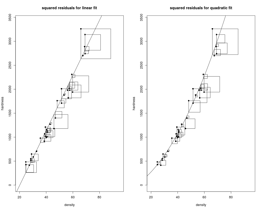
regr1.plot(hardness$density, hardness$hardness,
           resid.plot="square",
           main="squared residuals for linear fit",
           xlab="density", ylab="hardness",
           points.yhat=FALSE,
           xlim=c(20,95), ylim=c(0,3400))

regr1.plot(hardness$density, hardness$hardness,
           model=hardness.quad.lm,
           resid.plot="square",
           main="squared residuals for quadratic fit",
           xlab="density", ylab="hardness",
           points.yhat=FALSE,
           xlim=c(20,95), ylim=c(0,3400))

par(mfrow=c(1,1))

Results


R version 3.3.1 (2016-06-21) -- "Bug in Your Hair"
Copyright (C) 2016 The R Foundation for Statistical Computing
Platform: x86_64-pc-linux-gnu (64-bit)

R is free software and comes with ABSOLUTELY NO WARRANTY.
You are welcome to redistribute it under certain conditions.
Type 'license()' or 'licence()' for distribution details.

R is a collaborative project with many contributors.
Type 'contributors()' for more information and
'citation()' on how to cite R or R packages in publications.

Type 'demo()' for some demos, 'help()' for on-line help, or
'help.start()' for an HTML browser interface to help.
Type 'q()' to quit R.

> library(HH)
Loading required package: lattice
Loading required package: grid
Loading required package: latticeExtra
Loading required package: RColorBrewer
Loading required package: multcomp
Loading required package: mvtnorm
Loading required package: survival
Loading required package: TH.data
Loading required package: MASS

Attaching package: 'TH.data'

The following object is masked from 'package:MASS':

    geyser

Loading required package: gridExtra
> png(filename="/home/ddbj/snapshot/RGM3/R_CC/result/HH/regr1.plot.Rd_%03d_medium.png", width=480, height=480)
> ### Name: regr1.plot
> ### Title: plot x and y, with optional straight line fit and display of
> ###   squared residuals
> ### Aliases: regr1.plot
> ### Keywords: models regression
> 
> ### ** Examples
> 
> data(hardness)
> 
> ## linear and quadratic regressions
> hardness.lin.lm  <- lm(hardness ~ density,                data=hardness)
> hardness.quad.lm <- lm(hardness ~ density + I(density^2), data=hardness)
> 
> anova(hardness.quad.lm)  ## quadratic term has very low p-value
Analysis of Variance Table

Response: hardness
             Df   Sum Sq  Mean Sq F value    Pr(>F)    
density       1 21345674 21345674 815.923 < 2.2e-16 ***
I(density^2)  1   276041   276041  10.552  0.002669 ** 
Residuals    33   863325    26161                      
---
Signif. codes:  0 '***' 0.001 '**' 0.01 '*' 0.05 '.' 0.1 ' ' 1
> 
> par(mfrow=c(1,2))
> 
> regr1.plot(hardness$density, hardness$hardness,
+            resid.plot="square",
+            main="squared residuals for linear fit",
+            xlab="density", ylab="hardness",
+            points.yhat=FALSE,
+            xlim=c(20,95), ylim=c(0,3400))
> 
> regr1.plot(hardness$density, hardness$hardness,
+            model=hardness.quad.lm,
+            resid.plot="square",
+            main="squared residuals for quadratic fit",
+            xlab="density", ylab="hardness",
+            points.yhat=FALSE,
+            xlim=c(20,95), ylim=c(0,3400))
> 
> par(mfrow=c(1,1))
> 
> 
> 
> 
> 
> dev.off()
null device 
          1 
>