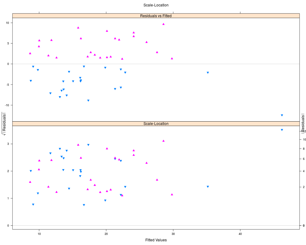
Draw plots of resid ~ y.hat and sqrt(abs(resid)) ~ y.hat

Description

Draw plots of resid ~ y.hat and sqrt(abs(resid)) ~ y.hat. This is a pair of lattice functions that duplicate the first and third panels of stats:::plot.lm.

Usage

residVSfitted(linearmodel, groups = (e >= 0), ...)
scaleLocation(linearmodel, groups = (e >= 0), ...)

Arguments

Value

"trellis" object.

Author(s)

Richard M. Heiberger <rmh@temple.edu>

Examples

data(fat)
fat.lm <- lm(bodyfat ~ abdomin, data=fat)

A <- residVSfitted(fat.lm, pch=c(25,24),
                   fill=trellis.par.get("superpose.symbol")$col[1:2])
B <- scaleLocation(fat.lm, pch=c(25,24),
                   fill=trellis.par.get("superpose.symbol")$col[1:2])
BA <- c("Scale-Location"=B,
        "Residuals vs Fitted"=update(A, scales=list(y=list(at=-100, alternating=3))),
        layout=c(1,2))
BA

BAu <-
  update(BA,
         ylab=c(B$ylab, A$ylab),
         ylab.right=c(B$ylab.right, A$ylab.right),
         xlab.top=NULL,
         between=list(y=1),
         par.settings=list(layout.widths=list(ylab.right=6))
         )

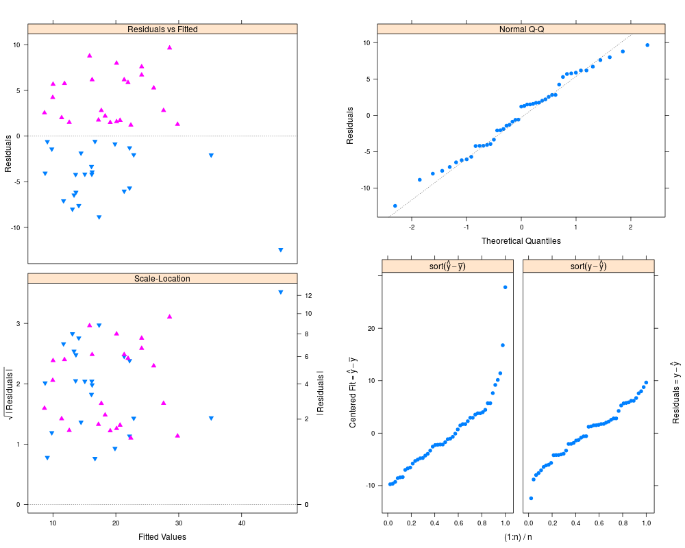
C <- diagQQ(fat.lm)

D <- diagplot5new(fat.lm)

print(BAu, split=c(1,1,2,1), more=TRUE)

print(update(c("Normal Q-Q"=C), xlab.top=NULL, strip=TRUE),
      ## split=c(2,1,2,2),
      position=c(.5, .54, 1, 1),  ## .54 is function of device and size
      more=TRUE)

print(update(D, xlab.top=NULL,
             strip=strip.custom(factor.levels=D$xlab.top),
             par.strip.text=list(lines=1.3)),
      ## split=c(2,2,2,2),
      position=c(.5, 0, 1, .57),  ## .57 is function of device and size
      more=FALSE)
## the .54 and .57 work nicely with the default quartz window on Mac OS X.

Results

R version 3.3.1 (2016-06-21) -- "Bug in Your Hair"
Copyright (C) 2016 The R Foundation for Statistical Computing
Platform: x86_64-pc-linux-gnu (64-bit)

R is free software and comes with ABSOLUTELY NO WARRANTY.
You are welcome to redistribute it under certain conditions.
Type 'license()' or 'licence()' for distribution details.

R is a collaborative project with many contributors.
Type 'contributors()' for more information and
'citation()' on how to cite R or R packages in publications.

Type 'demo()' for some demos, 'help()' for on-line help, or
'help.start()' for an HTML browser interface to help.
Type 'q()' to quit R.

> library(HH)
Loading required package: lattice
Loading required package: grid
Loading required package: latticeExtra
Loading required package: RColorBrewer
Loading required package: multcomp
Loading required package: mvtnorm
Loading required package: survival
Loading required package: TH.data
Loading required package: MASS

Attaching package: 'TH.data'

The following object is masked from 'package:MASS':

    geyser

Loading required package: gridExtra
> png(filename="/home/ddbj/snapshot/RGM3/R_CC/result/HH/residVSfitted.Rd_%03d_medium.png", width=480, height=480)
> ### Name: residVSfitted
> ### Title: Draw plots of resid ~ y.hat and sqrt(abs(resid)) ~ y.hat
> ### Aliases: residVSfitted scaleLocation
> ### Keywords: hplot
> 
> ### ** Examples
> 
> data(fat)
> fat.lm <- lm(bodyfat ~ abdomin, data=fat)
> 
> A <- residVSfitted(fat.lm, pch=c(25,24),
+                    fill=trellis.par.get("superpose.symbol")$col[1:2])
> B <- scaleLocation(fat.lm, pch=c(25,24),
+                    fill=trellis.par.get("superpose.symbol")$col[1:2])
> BA <- c("Scale-Location"=B,
+         "Residuals vs Fitted"=update(A, scales=list(y=list(at=-100, alternating=3))),
+         layout=c(1,2))
> BA
> 
> BAu <-
+   update(BA,
+          ylab=c(B$ylab, A$ylab),
+          ylab.right=c(B$ylab.right, A$ylab.right),
+          xlab.top=NULL,
+          between=list(y=1),
+          par.settings=list(layout.widths=list(ylab.right=6))
+          )
> 
> C <- diagQQ(fat.lm)
> 
> D <- diagplot5new(fat.lm)
> 
> print(BAu, split=c(1,1,2,1), more=TRUE)
> 
> print(update(c("Normal Q-Q"=C), xlab.top=NULL, strip=TRUE),
+       ## split=c(2,1,2,2),
+       position=c(.5, .54, 1, 1),  ## .54 is function of device and size
+       more=TRUE)
> 
> print(update(D, xlab.top=NULL,
+              strip=strip.custom(factor.levels=D$xlab.top),
+              par.strip.text=list(lines=1.3)),
+       ## split=c(2,2,2,2),
+       position=c(.5, 0, 1, .57),  ## .57 is function of device and size
+       more=FALSE)
> ## the .54 and .57 work nicely with the default quartz window on Mac OS X.
> 
> 
> 
> 
> 
> dev.off()
null device 
          1 
>