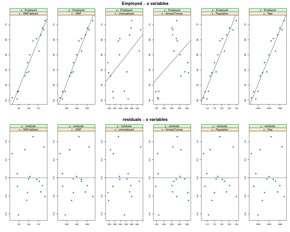
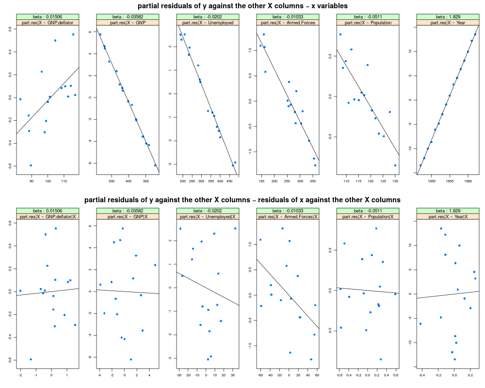
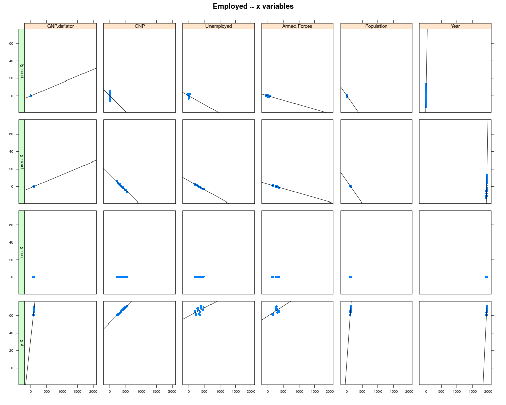
Residual plots for a linear model.

Description

Residual plots for a linear model. Four sets of plots are produced: (1) response against each of the predictor variables, (2) residuals against each of the predictor variables, (3) partial residuals for each predictor against that predictor ("partial residuals plots", and (4) partial residuals against the residuals of each predictor regressed on the other predictors ("added variable plots").

Usage

residual.plots(lm.object, X=dft$x,
               layout=c(dim(X)[2],1),
               par.strip.text=list(cex=.8),
               scales.cex=.6,
               na.action=na.pass,
               y.relation="free",
               ...)

Arguments

Value

A list of four trellis objects, one for each of the four sets of plots. The objects are named "y.X", "res.X" "pres.X", "pres.Xj". The default "printing" of the result will produce four pages of plots, one set per page. They are often easier to read when all four sets appear as separate rows on one page (this usually requires an oversize device), or two rows are printed on each of two pages.

Author(s)

Richard M. Heiberger <rmh@temple.edu>

References

Heiberger, Richard M. and Holland, Burt (2004b). Statistical Analysis and Data Display: An Intermediate Course with Examples in S-Plus, R, and SAS. Springer Texts in Statistics. Springer. ISBN 0-387-40270-5.

See Also

residual.plots.lattice

Examples

if.R(s={
     longley <- data.frame(longley.x, Employed = longley.y)
     },r={
     data(longley)
     })

longley.lm <- lm( Employed ~ . , data=longley, x=TRUE, y=TRUE)
## 'x=TRUE, y=TRUE' are needed to pass the S-Plus CMD check.
## They may be needed if residual.plots() is inside a nested set of
## function calls.

tmp <- residual.plots(longley.lm)

## print two rows per page
print(tmp[[1]], position=c(0, 0.5, 1, 1.0), more=TRUE)
print(tmp[[2]], position=c(0, 0.0, 1, 0.5), more=FALSE)
print(tmp[[3]], position=c(0, 0.5, 1, 1.0), more=TRUE)
print(tmp[[4]], position=c(0, 0.0, 1, 0.5), more=FALSE)

## print as a single trellis object
ABCD <- do.call(rbind, lapply(tmp, as.vector))
dimnames(ABCD)[[1]] <- dimnames(tmp[[1]])[[1]]
ABCD

Results

R version 3.3.1 (2016-06-21) -- "Bug in Your Hair"
Copyright (C) 2016 The R Foundation for Statistical Computing
Platform: x86_64-pc-linux-gnu (64-bit)

R is free software and comes with ABSOLUTELY NO WARRANTY.
You are welcome to redistribute it under certain conditions.
Type 'license()' or 'licence()' for distribution details.

R is a collaborative project with many contributors.
Type 'contributors()' for more information and
'citation()' on how to cite R or R packages in publications.

Type 'demo()' for some demos, 'help()' for on-line help, or
'help.start()' for an HTML browser interface to help.
Type 'q()' to quit R.

> library(HH)
Loading required package: lattice
Loading required package: grid
Loading required package: latticeExtra
Loading required package: RColorBrewer
Loading required package: multcomp
Loading required package: mvtnorm
Loading required package: survival
Loading required package: TH.data
Loading required package: MASS

Attaching package: 'TH.data'

The following object is masked from 'package:MASS':

    geyser

Loading required package: gridExtra
> png(filename="/home/ddbj/snapshot/RGM3/R_CC/result/HH/residual.plots.Rd_%03d_medium.png", width=480, height=480)
> ### Name: residual.plots
> ### Title: Residual plots for a linear model.
> ### Aliases: residual.plots
> ### Keywords: hplot regression
> 
> ### ** Examples
> 
> if.R(s={
+      longley <- data.frame(longley.x, Employed = longley.y)
+      },r={
+      data(longley)
+      })
> 
> longley.lm <- lm( Employed ~ . , data=longley, x=TRUE, y=TRUE)
> ## 'x=TRUE, y=TRUE' are needed to pass the S-Plus CMD check.
> ## They may be needed if residual.plots() is inside a nested set of
> ## function calls.
> 
> tmp <- residual.plots(longley.lm)
> 
> ## print two rows per page
> print(tmp[[1]], position=c(0, 0.5, 1, 1.0), more=TRUE)
> print(tmp[[2]], position=c(0, 0.0, 1, 0.5), more=FALSE)
> print(tmp[[3]], position=c(0, 0.5, 1, 1.0), more=TRUE)
> print(tmp[[4]], position=c(0, 0.0, 1, 0.5), more=FALSE)
> 
> ## print as a single trellis object
> ABCD <- do.call(rbind, lapply(tmp, as.vector))
> dimnames(ABCD)[[1]] <- dimnames(tmp[[1]])[[1]]
> ABCD
> 
> 
> 
> 
> 
> dev.off()
null device 
          1 
>