Supported by Dr. Osamu Ogasawara and  . . |
|
Last data update: 2014.03.03 |
Times series diagnostic plots for a structured set of ARIMA models.DescriptionTimes series diagnostic plots for a structured set of ARIMA models. Usage
tsdiagplot(x,
           p.max=2, q.max=p.max,
           model=c(p.max, 0, q.max), ## S-Plus
           order=c(p.max, 0, q.max), ## R
           lag.max=36, gof.lag=lag.max,
           armas=arma.loop(x, order=order,
               series=deparse(substitute(x)), ...),
           diags=diag.arma.loop(armas, x,
                                lag.max=lag.max,
                                gof.lag=gof.lag),
           ts.diag=rearrange.diag.arma.loop(diags),
           lag.units=ts.diag$tspar["frequency"],
           lag.lim=range(pretty(ts.diag$acf$lag))*lag.units,
           lag.x.at=pretty(ts.diag$acf$lag)*lag.units,
           lag.x.labels={tmp <- lag.x.at
                      tmp[as.integer(tmp)!=tmp] <- ""
                      tmp},
           lag.0=TRUE,
           main, lwd=0,
           ...)

acfplot(rdal, type="acf",
        main=paste("ACF of std.resid:", rdal$series,
                   "   model:",         rdal$model),
        lag.units=rdal$tspar["frequency"],
        lag.lim=range(pretty(rdal[[type]]$lag)*lag.units),
        lag.x.at=pretty(rdal[[type]]$lag)*lag.units,
        lag.x.labels={tmp <- lag.x.at
                      tmp[as.integer(tmp)!=tmp] <- ""
                      tmp},
        lag.0=TRUE,
        xlim=xlim.function(lag.lim/lag.units),
        ...)

aicsigplot(z, z.name=deparse(substitute(z)), series.name="ts",
           model=NULL,
           xlab="", ylab=z.name,
           main=paste(z.name,  series.name, model),
           layout=c(1,2), between=list(x=1,y=1), ...)

residplot(rdal,
          main=paste("std.resid:", rdal$series,
                     "   model:",  rdal$model),
          ...)

gofplot(rdal,
        main=paste("P-value for gof:", rdal$series,
                   "   model:",         rdal$model),
       lag.units=rdal$tspar["frequency"],
        lag.lim=range(pretty(rdal$gof$lag)*lag.units),
        lag.x.at=pretty(rdal$gof$lag)*lag.units,
        lag.x.labels={tmp <- lag.x.at
                      tmp[as.integer(tmp)!=tmp] <- ""
                      tmp},
        xlim=xlim.function(lag.lim/lag.units),
        pch=16, ...)
Arguments
Value
The other functions return Author(s)Richard M. Heiberger (rmh@temple.edu) References"Displays for Direct Comparison of ARIMA Models" The American Statistician, May 2002, Vol. 56, No. 2, pp. 131-138. Richard M. Heiberger, Temple University, and Paulo Teles, Faculdade de Economia do Porto. Richard M. Heiberger and Burt Holland (2004), Statistical Analysis and Data Display, Springer, ISBN 0-387-40270-5 See Also
Examples
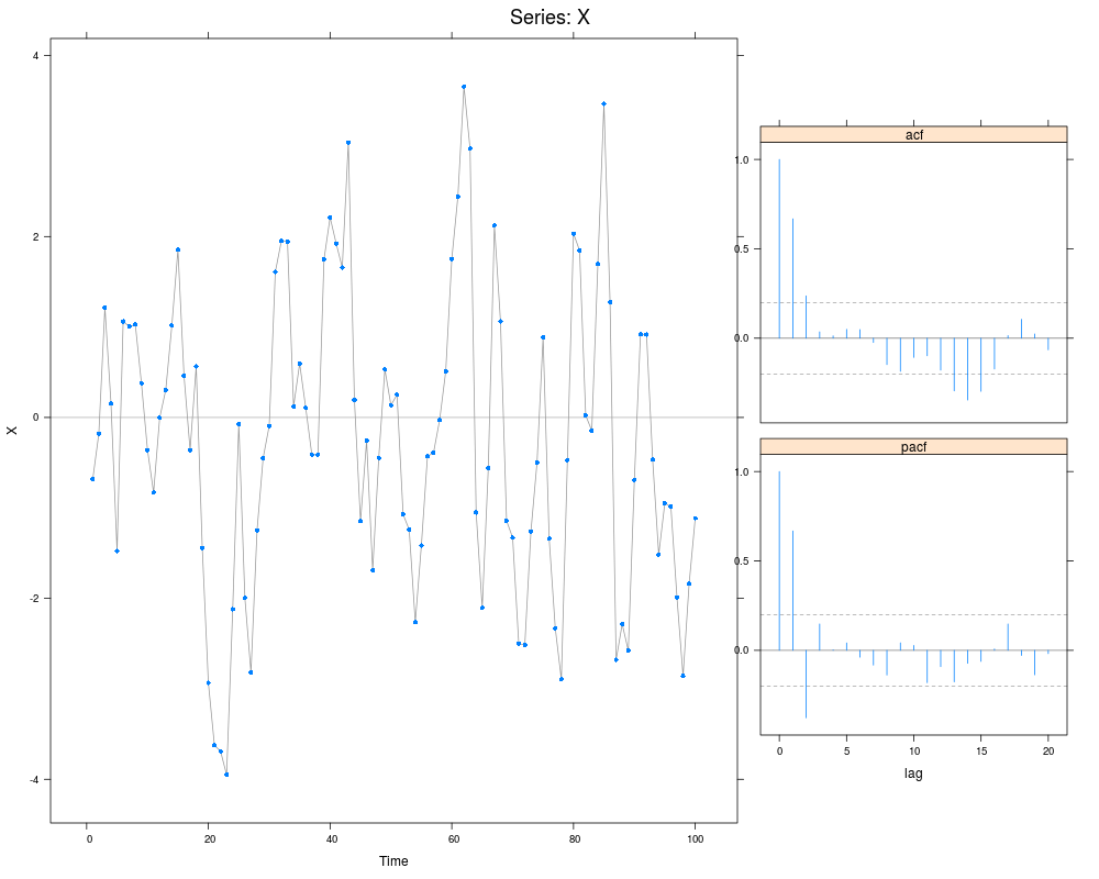
data(tser.mystery.X)
X <- tser.mystery.X
X.dataplot <- tsacfplots(X, lwd=1, pch.seq=16, cex=.7)
X.dataplot
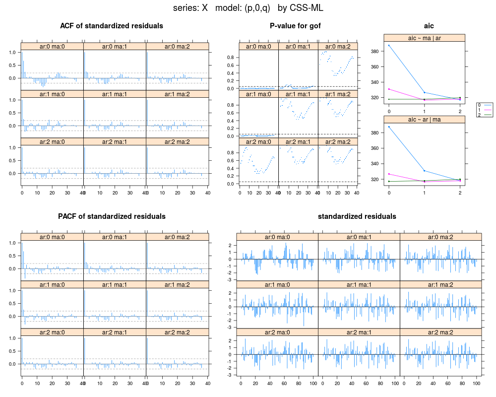
X.loop <- if.R(
s=
arma.loop(X, model=list(order=c(2,0,2)))
,r=
arma.loop(X, order=c(2,0,2))
)
X.dal <- diag.arma.loop(X.loop, x=X)
X.diag <- rearrange.diag.arma.loop(X.dal)
X.diagplot <- tsdiagplot(armas=X.loop, ts.diag=X.diag, lwd=1)
X.diagplot
X.loop
X.loop[["1","1"]]
Results
R version 3.3.1 (2016-06-21) -- "Bug in Your Hair"
Copyright (C) 2016 The R Foundation for Statistical Computing
Platform: x86_64-pc-linux-gnu (64-bit)

R is free software and comes with ABSOLUTELY NO WARRANTY.
You are welcome to redistribute it under certain conditions.
Type 'license()' or 'licence()' for distribution details.

R is a collaborative project with many contributors.
Type 'contributors()' for more information and
'citation()' on how to cite R or R packages in publications.

Type 'demo()' for some demos, 'help()' for on-line help, or
'help.start()' for an HTML browser interface to help.
Type 'q()' to quit R.

> library(HH)
Loading required package: lattice
Loading required package: grid
Loading required package: latticeExtra
Loading required package: RColorBrewer
Loading required package: multcomp
Loading required package: mvtnorm
Loading required package: survival
Loading required package: TH.data
Loading required package: MASS

Attaching package: 'TH.data'

The following object is masked from 'package:MASS':

    geyser

Loading required package: gridExtra
> png(filename="/home/ddbj/snapshot/RGM3/R_CC/result/HH/tsdiagplot.Rd_%03d_medium.png", width=480, height=480)
> ### Name: tsdiagplot
> ### Title: Times series diagnostic plots for a structured set of ARIMA
> ###   models.
> ### Aliases: tsdiagplot acfplot aicsigplot residplot gofplot
> ### Keywords: hplot
>
> ### ** Examples
>
> data(tser.mystery.X)
> X <- tser.mystery.X
>
> X.dataplot <- tsacfplots(X, lwd=1, pch.seq=16, cex=.7)
> X.dataplot
>
> X.loop <- if.R(
+                s=
+                arma.loop(X, model=list(order=c(2,0,2)))
+                ,r=
+                arma.loop(X, order=c(2,0,2))
+                )
> X.dal <- diag.arma.loop(X.loop, x=X)
> X.diag <- rearrange.diag.arma.loop(X.dal)
> X.diagplot <- tsdiagplot(armas=X.loop, ts.diag=X.diag, lwd=1)
> X.diagplot
>
> X.loop
$series
[1] "X"

$model
[1] "(p,0,q)"

$sigma2
         0        1        2
0 2.714968 1.434707 1.276545
1 1.500114 1.271072 1.262075
2 1.286423 1.260059 1.259868

$aic
         0        1        2
0 387.6657 326.6338 317.0996
1 330.9222 316.7015 318.0026
2 317.8579 317.8503 319.8347

$coef
              ar1        ar2       ma1        ma2  intercept
(0,0,0)        NA         NA        NA         NA         NA
(1,0,0) 0.6635554         NA        NA         NA -0.2744204
(2,0,0) 0.9134671 -0.3721161        NA         NA -0.2527722
(0,0,1)        NA         NA 0.7263795         NA -0.2568172
(1,0,1) 0.4298965         NA 0.5221491         NA -0.2628785
(2,0,1) 0.6213237 -0.1780866 0.3482906         NA -0.2571157
(0,0,2)        NA         NA 0.9272016 0.32957790 -0.2548033
(1,0,2) 0.2613548         NA 0.7056599 0.17340566 -0.2587636
(2,0,2) 0.5417462 -0.1478790 0.4279958 0.04825652 -0.2572223

$t.coef
              ar1        ar2       ma1       ma2  intercept
(0,0,0)        NA         NA        NA        NA         NA
(1,0,0) 9.0295264         NA        NA        NA -0.7683601
(2,0,0) 9.9262413 -4.0464280        NA        NA -1.0257358
(0,0,1)        NA         NA 13.203654        NA -1.2471457
(1,0,1) 3.8605613         NA  5.154041        NA -0.8827784
(2,0,1) 2.6785425 -0.9700575  1.526213        NA -0.9525257
(0,0,2)        NA         NA 10.628021 3.5060232 -1.0062817
(1,0,2) 1.0948883         NA  3.001941 0.8897271 -0.9135335
(2,0,2) 0.7891486 -0.4657525  0.624625 0.1266807 -0.9478341

> X.loop[["1","1"]]

Call:
arima(x = x, order = c(1, 0, 1))

Coefficients:
         ar1     ma1  intercept
      0.4299  0.5221    -0.2629
s.e.  0.1114  0.1013     0.2978

sigma^2 estimated as 1.271:  log likelihood = -154.35,  aic = 316.7
>
>
>
>
>
> dev.off()
null device
          1
>
|